
Merge and Manipulate Multiple Excel Sheets like a Pro
Working with multiple Excel sheets is common for many spreadsheet users. However, managing and consolidating data across worksheets and workbooks can be tedious and time-consuming…
Working with multiple Excel sheets is common for many spreadsheet users. However, managing and consolidating data across worksheets and workbooks can be tedious and time-consuming…
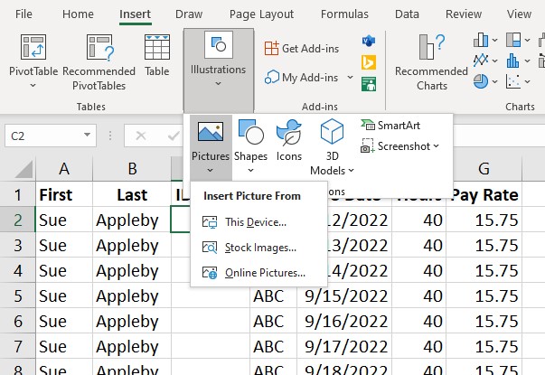
Placing images into your Excel worksheets can be beneficial for several reasons. For one, doing so can help pair product photos with their inventory descriptions…
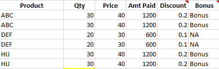
Excel tables come with a variety of features that make data recording and management a breeze. Instead of handling your data processes manually, save time…
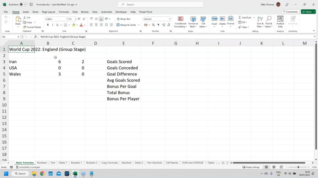
Addition, subtraction, multiplication, and division are essential mathematical functions that can be made easy by using Excel formulas. In Part 1 of this series, we covered…
Excel can be intimidating for people who have just been introduced to the program, but basic mathematical functions are relatively easy through Excel when you…
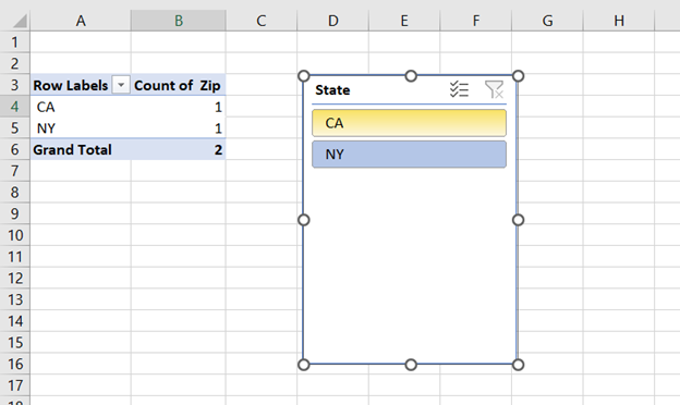
Are you looking for a way to filter your Excel pivot tables quickly? If so, then you need to learn about slicers! Slicers are a…
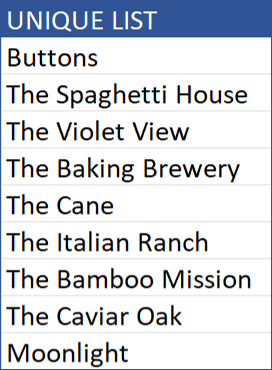
The Excel UNIQUE function returns a list of unique values in a list or range. Note: This function is currently available only to Microsoft 365…
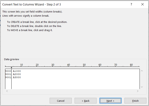
Do you have a list of data that you need to separate into columns in Excel? Maybe you have an address list with the city,…
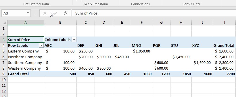
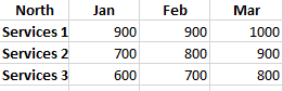
The pivot table in Excel is one of the most vital and versatile tools available. It allows you to look at your data from a…
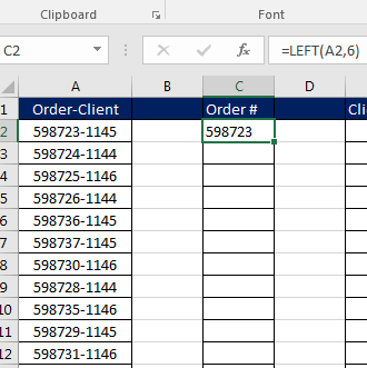
This demonstration covers how to use the LEFT and Right Functions in Excel. These are text functions. In the LEFT function, you can pull a…
Please confirm you want to block this member.
You will no longer be able to:
Please note: This action will also remove this member from your connections and send a report to the site admin. Please allow a few minutes for this process to complete.