The pivot table in Excel is one of the most vital and versatile tools available. It allows you to look at your data from a wide range of customizable views. In the following guide, we explore how to update the Pivot Table after the source data changes.

There are a variety of reasons you might need to update the pivot table. Maybe you get a weekly report that needs to be added each week. Instead of recreating the pivot table, you can simply refresh it. Maybe there were errors in the source data that needed to be corrected. Again, it’s simpler to refresh than to recreate.

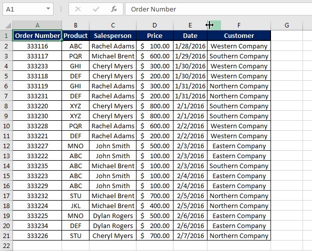
Let’s say you had the following spreadsheet:

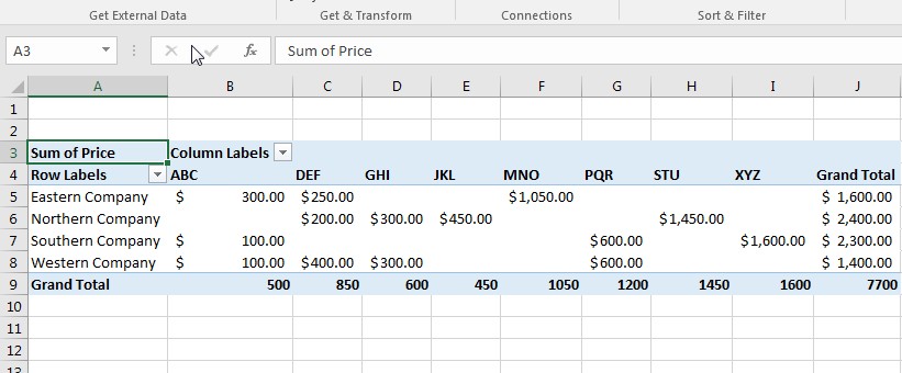
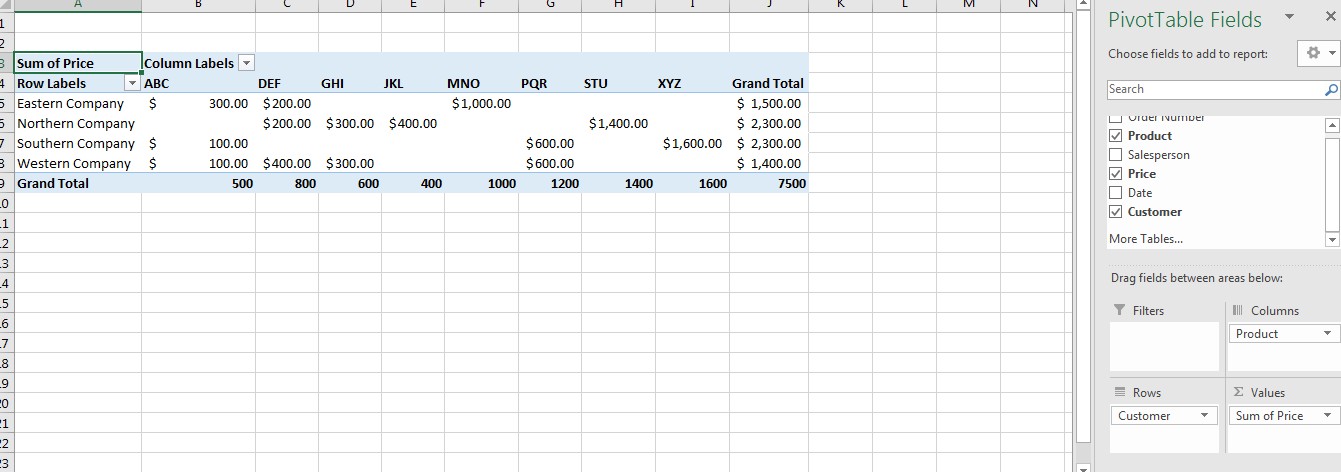
And you created this pivot table for it:

Then your manager informs you of a price correction on the last 4 items. They went up $50 each. For such a minor correction, it would be a waste of time to create a whole new pivot table. Instead, you will:

Make the source data correction
Go to the tab with the pivot table
Go to the Data tab on the Excel ribbon
Select Refresh

You can also use the keyboard shortcut Alt+F5 to perform this task.

As you can see in the animation above, once you apply the refresh option, the data in the table automatically updates with the source data corrections.

We hope you now feel comfortable making corrections to your pivot table source data and applying the refresh. This is one of many tools available to help you perfect your pivot tables.

Like Learn Excel Now? Follow us on social media and share our content with your networks! And don’t forget to sign up for the Newsletter

Kevin – Learn Excel Now

WELCOME BACK!

Reset Password