
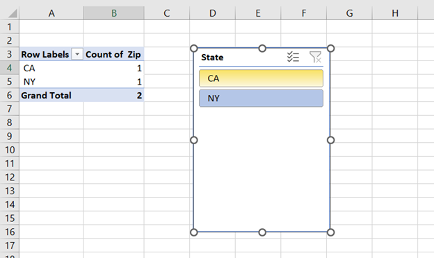
Merge and Manipulate Multiple Excel Sheets like a Pro
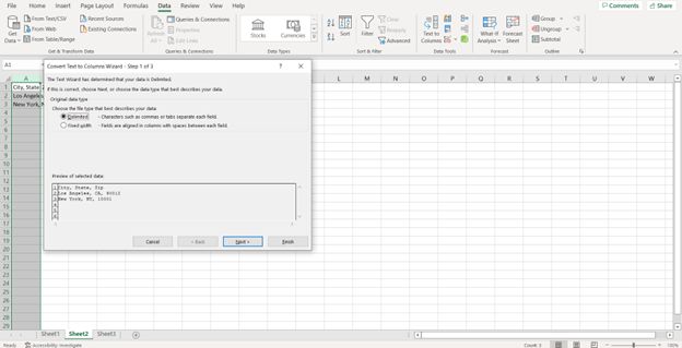
Working with multiple Excel sheets is common for many spreadsheet users. However, managing and consolidating data across worksheets and workbooks can be tedious and time-consuming…
Working with multiple Excel sheets is common for many spreadsheet users. However, managing and consolidating data across worksheets and workbooks can be tedious and time-consuming…

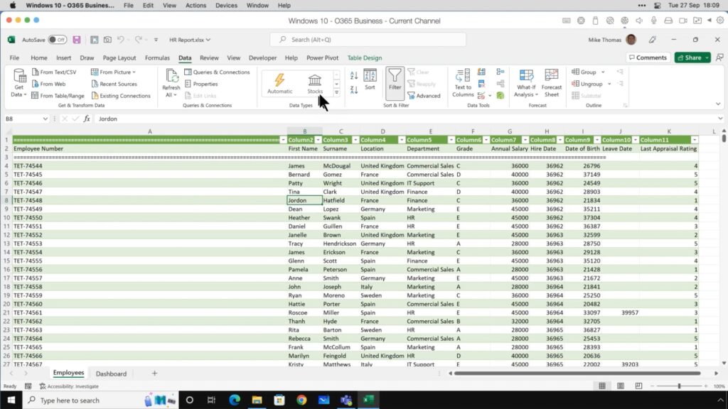
Data is the foundation of any analysis, decision-making process, or business strategy. However, raw data seldom comes perfectly organized and error-free. That’s where data cleaning…
Serial numbers are an essential part of many datasets because you can use them to identify specific entries in your sheet. Adding them manually can…
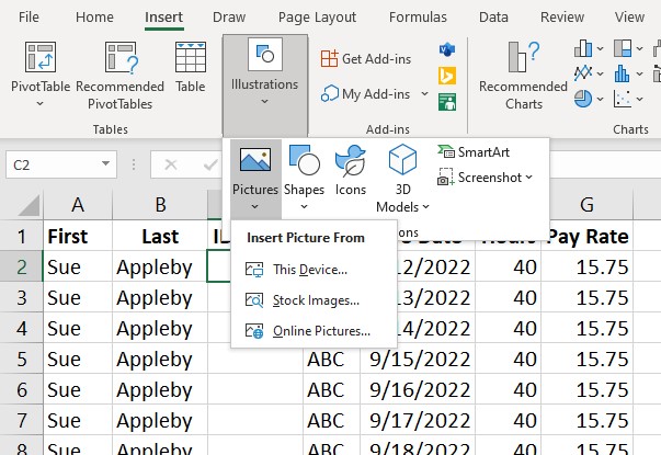
Placing images into your Excel worksheets can be beneficial for several reasons. For one, doing so can help pair product photos with their inventory descriptions…
The XLOOKUP function is relatively new, and it was introduced to provide solutions for some of the issues that commonly occur when using the VLOOKUP…
HLOOKUP is a function that Excel users can key in to look up and retrieve data from a specific row in a table. This function…
VLOOKUP is a relatively common Excel function that aims to simplify locating a specific piece of information located within a spreadsheet. For example, if you…
Excel tables come with a variety of features that make data recording and management a breeze. Instead of handling your data processes manually, save time…
Most working professionals want to save time when writing reports and copying data into spreadsheets, yet worrying about making mistakes can slow progress to a…
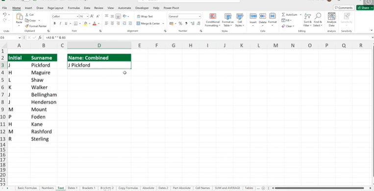
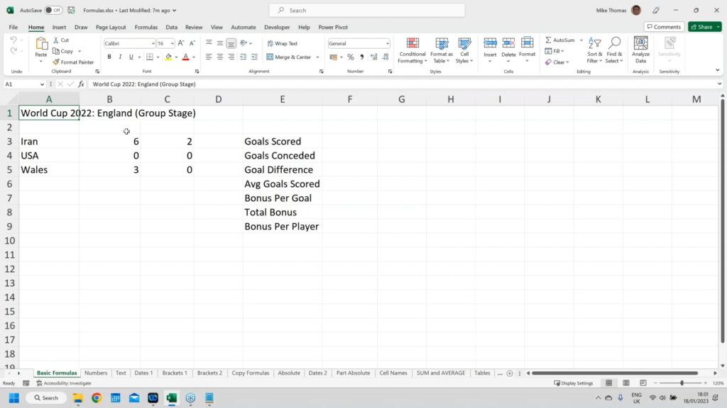
Learning a selection of Excel formulas can take your reports to the next level. Mastering a few tips and tricks can not only save time…
Please confirm you want to block this member.
You will no longer be able to:
Please note: This action will also remove this member from your connections and send a report to the site admin. Please allow a few minutes for this process to complete.