
Merge and Manipulate Multiple Excel Sheets like a Pro
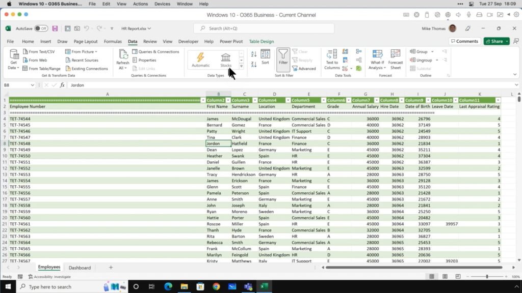
Working with multiple Excel sheets is common for many spreadsheet users. However, managing and consolidating data across worksheets and workbooks can be tedious and time-consuming…
Working with multiple Excel sheets is common for many spreadsheet users. However, managing and consolidating data across worksheets and workbooks can be tedious and time-consuming…
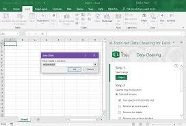
Data is the foundation of any analysis, decision-making process, or business strategy. However, raw data seldom comes perfectly organized and error-free. That’s where data cleaning…
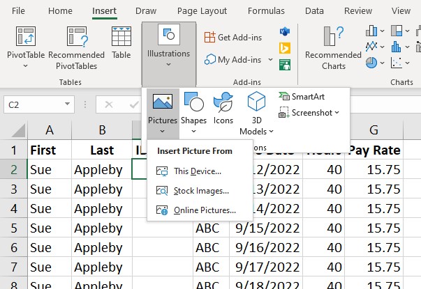
Placing images into your Excel worksheets can be beneficial for several reasons. For one, doing so can help pair product photos with their inventory descriptions…
The XLOOKUP function is relatively new, and it was introduced to provide solutions for some of the issues that commonly occur when using the VLOOKUP…
HLOOKUP is a function that Excel users can key in to look up and retrieve data from a specific row in a table. This function…
Excel tables come with a variety of features that make data recording and management a breeze. Instead of handling your data processes manually, save time…
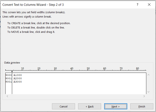
Do you have a list of data that you need to separate into columns in Excel? Maybe you have an address list with the city,…
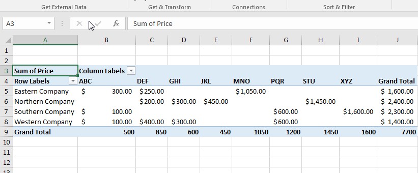
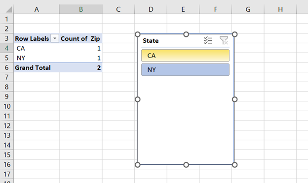
The pivot table in Excel is one of the most vital and versatile tools available. It allows you to look at your data from a…
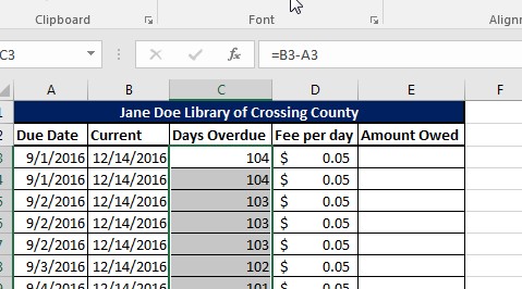
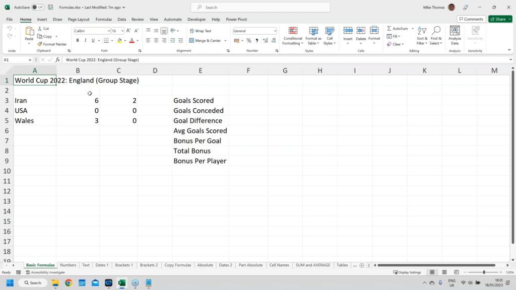
Excel has several built-in date functions you can use to quickly find important information. These are known as Excel date calculations. Today, we will focus…
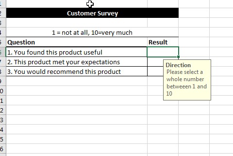
Excel data validation allows you to set specific criteria for the type of data that can be entered into a cell or group of cells.…
Please confirm you want to block this member.
You will no longer be able to:
Please note: This action will also remove this member from your connections and send a report to the site admin. Please allow a few minutes for this process to complete.