Learn Excel Now

Conquer the Fear of Excel

  • Home
    • Our Team
  • Training
    • Custom Training
      • Custom Virtual Group Training
      • Custom Onsite Group Training
      • Consulting Services
    • Excel
    • MS Office
    • Outlook
    • PowerPoint
    • Word
    • OneDrive
    • Google
  • All-Access
  • eLearning
    • Excel Foundations
    • Micro Courses
      • Simply Excel
      • Simply Excel Pt. II
  • Resources
    • Contact
    • FAQ
    • New User Onboarding
  • Login

Excel Pivot Tables: Using Slicers to Filter Data

September 30, 2022 by Austin Chia

Are you looking for a way to filter your Excel pivot tables quickly? If so, then you need to learn about slicers! Slicers are a great way to control the data that is displayed in your pivot table.

In this blog post, we will introduce you to pivot table slicers and show you how to use them through a step-by-step tutorial.

So, if you want to learn how to use slicers with pivot tables, keep reading!

What Are Pivot Table Slicers?

Pivot table slicers are a new feature only found in versions from Excel 2010 onward. They allow you to quickly filter pivot table data by clicking on a value in the slicer.

Why Use Pivot Table Slicers?

Pivot table slicers are a great way to filter pivot table data in Excel. Slicers are an alternative to the default filters in Excel.

They are easy to use and they provide a quick way to change the data that is displayed in your pivot table. You’ll be able to mine data for useful business insights.

Another advantage of using slicers is that they can be used to filter multiple pivot tables at the same time. This is because slicers are connected to pivot tables.

Therefore, if you have multiple pivot tables in your workbook, you can use a slicer to filter all of them at the same time. This can save you a lot of time if you need to regularly filter pivot table data.

When Should Pivot Table Slicers Be Used?

Pivot table slicers should be used when you need to quickly filter pivot table data. They are handy if you have multiple pivot tables in your workbook.

They’re also a great way to filter data when creating an Excel dashboard for your Excel project.

With the use of pivot table slicers in Excel, you’ll get to dig deeper into your data and visualize them better through charts.

Although not as powerful as the filters available in other data analysis tools like Tableau, slicers are easy to create and implement in your work!

How Do Pivot Table Slicers Work?

Pivot table slicers work by connecting to pivot tables. When you create a slicer, you need to specify which pivot table it should be connected to. Once a slicer is connected to a pivot table, it can be used to filter the data in that pivot table.

If you have multiple pivot tables in your workbook, you can connect a slicer to all of them. This will allow you to quickly filter the data in all of the pivot tables at the same time.

How To Use Pivot Table Slicers to Filter Data

Now that you know the basics of using pivot table slicers, let’s take a look at how to use them with a pivot table. We will walk you through the process step-by-step so that you can see how it’s done.

To start, select the pivot table with which you want to use the slicer. Then, click on the “Insert” tab and then click on “Slicer.”

In the “Select a slicer” window, select the field that you want to use as a slicer. For this example, we will use the “State” field.

Next, click “OK.” Your pivot table should now have a slicer associated with it. To use the slicer, simply click on the items that you want to include in your pivot table.

For example, if you only want to see data for the states of “CA” only, click on “CA”. The pivot table will update to only include data for that state.

And if you want to filter and include bot, hold Shift and click both “CA” and “NY”. The pivot table will update to only include data for those two states.

By using this slicer, you’re able to quickly switch between states by selecting the values you need. This can be great when presenting important data using your pivot table.

Rather than just using the regular filters in the pivot table slicers give you a more intuitive way to interact with your data!

Having this knowledge of using slicers in your pivot tables is an essential skill in data analytics in business, where presentation summaries are used in day-to-day operations.

Key Takeaways:

  • Pivot table slicers are a great way to quickly filter pivot table data.
  • They’re easy to use and can be connected to multiple pivot tables.
  • You can use them to filter data by region, sales, criteria, etc.

Conclusion

As you can see, pivot table slicers are a great way to quickly filter your data. So, if you haven’t already started using them, we encourage you to do so!

Thanks for reading!

Enjoyed this basic tutorial on separating data? Having basic training in Microsoft Excel is important for success in many jobs. If you want to learn more about how to use Excel, check out the other blog posts or sign up for one of our Excel trainings!

Like Learn Excel Now? Follow us on social media and share our content with your networks! And don’t forget to sign up for the Newsletter

Author Bio

Austin Chia is the Founder of Any Instructor. A data analytics and Excel enthusiast, he seeks to help others learn more about Excel and anything related to analytics and tech. He has experience as a data analyst and data scientist in healthcare and research.

Excel Pivot Table Tips: Refreshing the Table After Source Data Changes

February 1, 2017 by Tyrone Pernsley

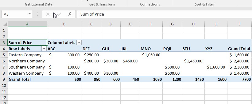
The pivot table in Excel is one of the most vital and versatile tools available. It allows you to look at your data from a wide range of customizable views. In the following guide, we explore how to update the Pivot Table after the source data changes.

There are a variety of reasons you might need to update the pivot table. Maybe you get a weekly report that needs to be added each week. Instead of recreating the pivot table, you can simply refresh it. Maybe there were errors in the source data that needed to be corrected. Again, it’s simpler to refresh than to recreate.

Let’s say you had the following spreadsheet:

Refreshing Pivot Table Image 1

And you created this pivot table for it:

Refreshing Pivot Table Image 2

Then your manager informs you of a price correction on the last 4 items. They went up $50 each. For such a minor correction, it would be a waste of time to create a whole new pivot table. Instead, you will:

  • Make the source data correction
  • Go to the tab with the pivot table
  • Go to the Data tab on the Excel ribbon
  • Select Refresh

Refreshing Pivot Table for New Data

You can also use the keyboard shortcut Alt+F5 to perform this task.

As you can see in the animation above, once you apply the refresh option, the data in the table automatically updates with the source data corrections.

We hope you now feel comfortable making corrections to your pivot table source data and applying the refresh. This is one of many tools available to help you perfect your pivot tables.

Like Learn Excel Now? Follow us on social media and share our content with your networks! And don’t forget to sign up for the Newsletter

Kevin – Learn Excel Now

Sorting Data with Excel Pivot Tables

March 9, 2016 by Tyrone Pernsley

The Pivot Table is one of the most useful features in Excel. Sorting data with  Excel Pivot Tables allows you to examine your data from multiple points of view for better summary and analysis. You can sort data, count totals, averages, percentages, etc. In addition to giving you the ability to organize your data, Pivot Tables also makes your data more presentable.

Creating a PivotTable

Sorting Data with Excel Pivot Tables GIF 1

Once you have highlighted the data that you want in your Pivot Table report, go to the “Insert” tab and click on “Pivot Table.” You can then be able to choose to create the Pivot Table report on a new page or keep it on the same page as your data. The Pivot Table that is generated will be blank, so you have to pick which values you want and where you want them. You can arrange your data in rows or columns and include sums of different data series. To do this, you simply use the Pivot Table Field List on the right to drag and drop fields to the area where you want them to go. Your Pivot Table will then be generated and then you can sort and organize it.

PivotTable image1

Sorting Data

PivotTables can be used to organize and sort all kinds of data. Some examples include:

  • Alphabetically
  • Numerically
  • By dates and time

The options for selecting which data to look will be affected by the row and column labels in the original data set. For example, if you have a list of purchases and want to organize them by date, you can move the two column labels into the Pivot Table fields.

In the Pivot Table report, click on the drop-down arrow next to “Row Labels” or “Column Labels,” then select how you want your data to be sorted. If all of your values are words, you’ll be able to sort the data alphabetically from A to Z or from Z to A. For numeric values, you can sort it from smallest to largest or from largest to smallest. For times and dates, you can sort form oldest to newest or newest to oldest. You can also drag and move data to sort it in any way you want.

Sorting Data with Excel Pivot Tables GIF 2

Once you have your data organized into the proper fields, you can begin to summarize the findings for improved decision-making.

We here at Learn Excel Now hope you enjoyed this quick guide on sorting data with Pivot Tables. It is our desire to bring you the best advice and training available so you can effectively and efficiently use your Excel tools.

Liked this sorting data with Excel Pivot Tables quick tip? Have questions? Leave your comments below; we’d love to hear from you.

Getting Social with Excel: Spread the word and share the knowledge!

Kevin – Learn Excel Now

All Access Subscription
Our 1-year all-access subscription provides step-by-step guidance for mastering Microsoft Office applications, with workshops, exercises and quick reference eGuides. It's perfect for anyone that needs to brush up on certain skills or even folks who need to learn the programs - from a beginner’s level.
Excel Foundations
Take the fear out of Excel with this 20 module self-paced training course. You will cover the most essential topics to develop a solid foundation of Excel or a lifetime of mastery.

Learn Excel Now helps you conquer the fear of Excel. By providing self-paced and instructor-led training and free strategies and guides, we leave no Excel mystery unsolved.

  • Home
  • Training
  • All-Access
  • Excel Foundations
  • Resources

Connect with Us

  • Facebook
  • Linkedin

Contact

Learn Excel Now
questions@learnexcelnow.com
1-484-259-7664 or 1-800-964-6033
660 American Ave
Suite 203
King of Prussia, PA 19406

Microsoft® Office Excel® is a registered trademark of the Microsoft Corporation in the United States and other countries. All rights reserved.

Copyright © 2023 ­Learn Excel Now

Terms of Service

Privacy Policy

Copyright © 2023 · News Pro Theme on Genesis Framework · WordPress · Log in

WELCOME BACK!

Enter your username and password below to log in

Forget Your Username or Password?

Reset Password

Lost your password? Please enter your username or email address. You will receive a link to create a new password via email.

Log In