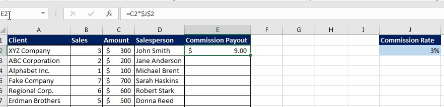
Creating Basic Formulas Part 2: Multiplication

December 23, 2022 by Madeleine Moucheron

Addition, subtraction, multiplication, and division are essential mathematical functions that can be made easy by using Excel formulas.

In Part 1 of this series, we covered creating basic addition and subtraction formulas in Excel. This week we’ll tackle how to multiply with the program.

Multiplication Formula

Like adding and subtracting, multiplying cells can be done by typing in the totals or by using the cell names. Let’s say that you want to multiply F4 and F8, which will be 12 and 3 for this example.

You can name the cells in the formula =F4*F8, or you can type the totals into the formula =12*3.

The PRODUCT function can also be used to multiply different cells. To use it, click on the cell where you want your total to appear, then type in “=product” and choose the PRODUCT function. Then, as with using the =SUM function, select the cells you want to multiply and hit Enter.

We at Learn Excel Now hope you feel comfortable creating addition formulas with Excel. Next week, we’ll wrap up this series with how to divide in Excel so stay tuned!

Like Learn Excel Now? Follow us on social media and share our content with your networks!

Creating Basic Formulas Part 1: Addition and Subtraction

December 15, 2022 by Madeleine Moucheron

Excel can be intimidating for people who have just been introduced to the program, but basic mathematical functions are relatively easy through Excel when you know the right formulas.

To begin, we’ll just cover the basic formulas for now: Addition, Subtraction, Multiplication, and Division.

Let’s begin with Addition and Subtraction.

Addition Formula

The basic way to add numbers from different cells on your Excel spreadsheet involves writing the first cell name (the column and row letter and number), then the plus (+) sign, then the next cell name. For example, =C5+C8.

If you want, you can also combine the numbers in the cells you want so that you don’t have to type in the cell names. This can be done by typing the list of numbers into the upper input bar. For example, =5+3+4+12+9 (let’s say these are the numbers in E3 to E7).

You can also use the SUM function by typing “=sum” into the area where your totals will be recorded. Once the SUM function populates, you can select all of the cells you want to include in the addition formula.

Subtraction Formula

Much like creating an addition formula, subtraction can be done by typing in the first cell name you want to use, then the subtraction (-) sign, then the next cell name. For example, =B4-B2.

You can also subtract the number totals the same way you can with addition. However, there is no subtraction function in Excel.

We at Learn Excel Now hope you feel comfortable creating addition formulas with Excel. Next week, we will cover how to multiply in Excel so stay tuned!

Like Learn Excel Now? Follow us on social media and share our content with your networks!

Excel Basics: How To Separate Text Into Columns

August 22, 2022 by Austin Chia

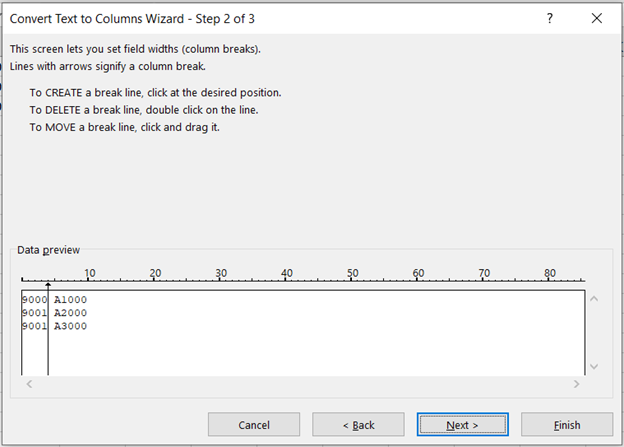
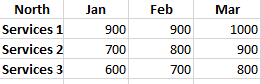
Do you have a list of data that you need to separate into columns in Excel? Maybe you have an address list with the city, state, and zip code all in one column. Or maybe you have a list of product SKUs and want to separate them into individual columns.

Well, before you can start applying all your Excel formulas, you’ll need to get your data all cleaned up. Data is typically cleaned by data engineers but if you’re working with financial data that mostly live within Excel databases, you’ll have to clean it yourself.

In this blog post, I will show you how to use the text to columns wizard in Excel to easily separate text into columns.

I will explain how to use the wizard by both delimiter and fixed width. So whether your data is separated by commas, tabs, or spaces, I will show you how to get it into neat and tidy columns!

Let’s get started!

How Do You Separate Text Into Columns in Excel?

Have you ever tried to filter your data in Excel only to find that all of your data ended up in one column? Before you try out these database tips in Excel, you might want to separate your data into columns first!

It can be frustrating, but luckily there is a tool that can help. The text to columns wizard in Excel allows you to easily separate text into multiple columns.

There are two main ways to use the text to columns wizard: by a delimiter and by fixed width.

If your data is separated by a specific character, such as a comma or tab, then you would use the delimiter option. For example, if your data looks like this:

You would use a comma as your delimiter.

If your data is not separated by a specific character, but you want to split it into columns of equal width, then you would use the fixed width option.

For example, if your data looks like this:

You would use fixed width to split the text into columns.

How To Use The Delimiter Option to Separate Text in Excel

Let’s say you have a list of addresses in one column and you want to separate them into individual columns for the city, state, and zip code. To do this, we would use the delimiter option.

First, highlight the column of data that you want to split. Then, go to the Data tab and click Text to Columns.

In the Convert Text to Columns Wizard, select Delimited and click Next.

On the next page, check the box next to Comma and clear any other boxes that are checked. Then, click Next.

On the next page, you will see a preview of how your data will look when it is split into columns. If everything looks good, click Finish.

And that’s it! Your text should now be split into columns.

End Result

Now that your data is arranged neatly into separate columns, your data format is more suited for further analysis using pivot tables!

How To Use The Fixed Width Option to Separate Text in Excel

If you want to split your text by fixed width, the process is similar. Highlight the column of data that you want to split and go to the Data tab. Click Text to Columns.

In the Convert Text to Columns Wizard, select Fixed Width and click Next.

On the next page, you will see a preview of how your data will look when it is split into columns. Place a break in between each column where you want to split the text. Then, click Next.

On the next page, you will see a preview of how your data will look when it is split into columns. If everything looks good, click Finish.

And that’s it! Your text should now be split into columns.

End Result

I hope this blog post was helpful in showing you how to use the text to columns wizard in Excel. Do consider using this simple but powerful tool in your next data mining or Excel project.

Key Takeaways:

– The text to columns wizard in Excel allows you to easily separate text into multiple columns.

– There are two main ways to use the text to columns wizard: by delimiter and by fixed width.

– If your data is separated by a specific character, such as a comma or tab, then you would use the delimiter option.

– If your data is not separated by a specific character, but you want to split it into columns of equal width, then you would use the fixed width option.

– To use the text to columns wizard, highlight the column of data that you want to split and go to the Data tab. Click Text to Columns. Then, follow the instructions in the wizard.

– Your text should now be split into columns.

Thanks for reading!

Enjoyed this basic tutorial on separating data? Having basic training in Microsoft Excel is important for success in many jobs. If you want to learn more about how to use Excel, check out the other blog posts or sign up for one of our Excel training workshops!

Like Learn Excel Now? Follow us on social media and share our content with your networks! And don’t forget to sign up for the Newsletter

Author Bio

Austin Chia is the Founder of Any Instructor. A data analytics and Excel enthusiast, he seeks to help others learn more about Excel and anything related to analytics and tech. He has experience as a data analyst and data scientist in healthcare and research.

How to Use the Excel MEDIAN Function

November 9, 2016 by Tyrone Pernsley

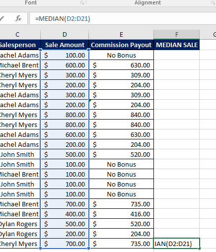
In this week’s Excel tip, we cover how to use the Excel MEDIAN function. The MEDIAN function is used the return the median value within the defined range.

For this demonstration, we will use the follow example:

The task assigned for this spreadsheet was to find the median sale amount. To do this, we will use the MEDIAN formula:

=MEDIAN(Number1, [number2]..)

Since the goal is to find the median in a single range, the formula becomes:

=MEDIAN(D2:D21)

And once you enter the formula, you get the return value:

Since there were 20 cells within the range, the formula found the average between two middle values.

We at Learn Excel Now hope you feel comfortable using the MEDIAN function now.

Like Learn Excel Now? Follow us on social media and share our content with your networks! And don’t forget to sign up for the Newsletter

Kevin – Learn Excel Now

How to Show Formulas in Excel

October 26, 2016 by Tyrone Pernsley

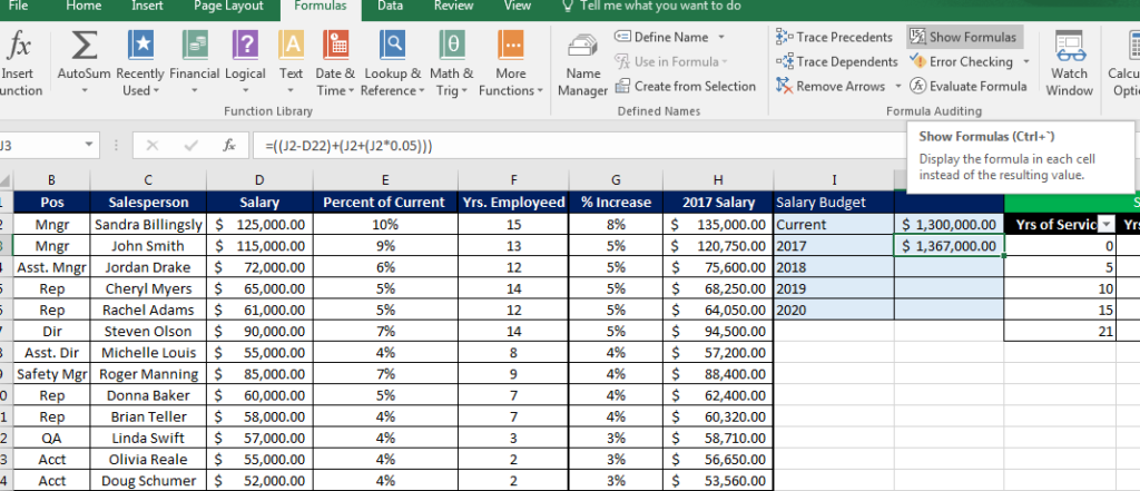
In this week’s blog post, we cover how to show formulas in Excel. This convenient feature is ideal for identifying which cells contain formulas and what those formulas are.

John was recently hired in human resources for a large sales firm. His job is to manage the salaries for the sales, accounting and shipping departments. Once hired, he received the following spreadsheet from his predecessor.

He was not a fan of the layout and functionality of the spreadsheet. He wanted to change it around to make more sense to him and to give him more control over the data. However, he knew some of the cells contained formulas and moving things around could throw off the whole spreadsheet.

So, his first step in taking ownership over the spreadsheet was to identify which cells are using formulas. There are two ways to show formulas in Excel:

On the Excel Ribbon, go to the Formulas tab and click on the Show Formulas button
Keyboard shortcut: Ctrl+` (Control and the accent mark, aka Tilde)

The following Gif provides a demo using the first option:

However, using the Ctrl+` would result in the same.

We at Learn Excel Now hope you now feel confident finding the formulas in your spreadsheet.

Like Learn Excel Now? Follow us on social media and share our content with your networks! And don’t forget to sign up for the Newsletter

Kevin – Learn Excel Now

Excel Formulas: Using Trace Dependents to Find Data Solutions

October 19, 2016 by Tyrone Pernsley

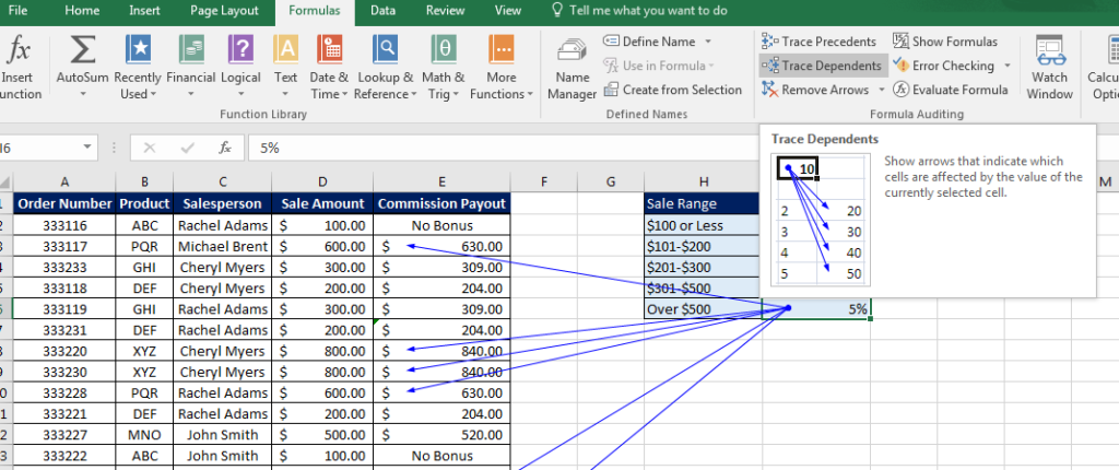
In last week’s post, we covered how to use Trace Precedents to find and resolve formula errors. In this week’s follow up, we cover how to use trace dependents to see which formulas use the data contained in a particular cell.

Donna was recently sent her company’s sales spreadsheet:

The commission rate was set to 5% for sales over $500. Her boss wants to increase the rate to 6%. She has two tasks: identify which sales will be affected by the increase and how many sales are over $500.

There are a number of ways Donna can find the data she needs. She could manually count the sales columns. She could use a lookup function. However, she prefers to have a clear visual to show which ones are the important ones.

By using Trace Dependents, she can quickly see which bonuses are for sales over $500, allowing her to determine which ones will be impacted and how many there are. Here is how she used Trace Dependents:

Find the cell with the relevant data – in this case, the 5% in the commission table (Cell I6)
While you are on that cell, click the Formulas tab in the Ribbon
Under the Formula Auditing menu, click on Trace Dependents
The arrows will point to every cell using a formula which uses I6

We at Learn Excel Now hope you feel confident using Trace Dependents now. There are many times and reasons this tool will come in handy.

Like Learn Excel Now? Follow us on social media and share our content with your networks! And don’t forget to sign up for the Newsletter

Kevin – Learn Excel Now

Excel Formulas: Using Trace Precedents to Find & Resolve Errors

October 12, 2016 by Tyrone Pernsley

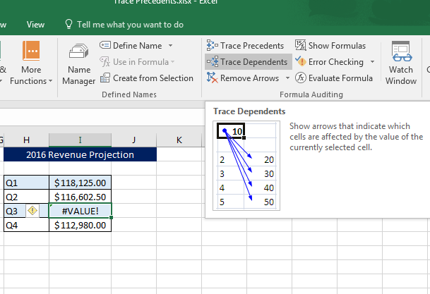
The power of Excel comes from the ability to do complicated calculations using formulas and functions. Sometimes, though, there are errors in formulas that give an error message or return the wrong value. In those instances, Excel also provides tools to resolve errors and check your work. One such tool is trace precedents.

The trace precedents tool finds any and all cells that provide information for the target cell. For example, if you summed up the totals in A1 and B1 into cell C1, both cells A1 and B1 would be precedents for C1.

Some errors in Excel are related to one or more precedent cells giving information that throws off the formula. Trace precedents is a great way to determine if there is a cell causing the issue, and if so, which cell needs to be corrected

For an example of using trace precedents to resolve formula errors, we will use the following spreadsheet:

In this instance, the table is using a simple formula to create revenue projections. The previous year’s quarterly total is increased by the projected growth of 5%. As you can see though, the Q3 project, cell I5, is showing an error message.

So, we will use the trace precedents tool to see if there are any cells causing the issue:

In the demo above, the error was created because one of the cells was incorrect. Instead of the cell containing the percentage amount (5% in cell F4) it was trying to pull the definition of that number one cell above (F3).

The issue could have been caused by simple human error. The person entering the formulas could have simply clicked on the wrong cell.

Once the wrong cell was identified using trace precedents, it was a simple matter of editing the formula to the correct cell and the error was resolved.

There are many instances where this tool could come in handy. Aside from resolving errors, sometimes you might just want to see which cells feed into a formula.

Stay tuned for part 2 next week on Trace Dependents!

We here at Learn Excel Now hope you now feel confident using the trace precedents tool to resolve formula issues.

Like Learn Excel Now? Follow us on social media and share our content with your networks! And don’t forget to sign up for the Newsletter

Kevin – Learn Excel Now

Excel IF Statements Part 3 – Nested IF Statements

August 10, 2016 by Tyrone Pernsley

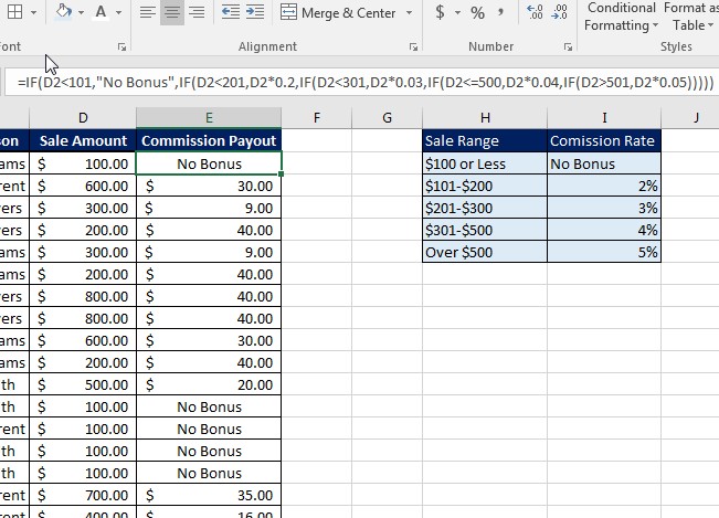
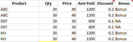
In this week’s IF statement series, we are covering Nested IF Statements. This convenient formula allows you to return values based on multiple logic tests built into – or nested – in the formula itself. We will explore several uses of nested IF statements in demonstrations below.

Syntax of Nested IF Statements

When you write a nested IF statement, you are essentially saying “If true, do this, if true, do this, if true, do this…if false, then do you this.” You can nest up to seven IF criteria within the formula.

The syntax for nested IF Statements is:

=IF(True-This,IF(True, this,IF(True,this,IF(True,This,IF(False,this))))

Notice: For each new IF statement, you open a new parenthesis, however, the parenthesis closing all come at the end of the formula.

Uses for Nested IF Statements

There are many reasons to use nested IF statements and you will have to determine the best situations to employ them. For the purposes of demonstration, we will use nested IF statements to calculate commission rates based on a sliding scale and salary increases based on years of service.

Calculating Commission on a Sliding Scale

If you remember our Simple IF Statements from last week, we used a single IF condition to return a flat bonus rate or determine No Bonus. But, what if there is a sliding scale? By nesting several IF statements together, you can create a dynamic formula that returns the commission amount based on a sliding scale.

Let’s say you had the following spreadsheet:

You can see the sliding scale in the table to the right. To write this scale into a nested IF statement you would write it as:

=IF(D2<101,”No Bonus”,IF(D2<201,D2*0.03,IF(D2<301,D2*0.03,IF(D2<=500,D2*0.04,IF(D2>501,D2*0.05)))))

Here, what you are saying is: IF the amount in column D is less than 101, return the value No Bonus, IF it’s less than 201, times the amount by 2% (0.02), IF less than 301, times it by 3%, IF less than or equal to 500, times it by 4%, and if it’s greater than 501, times it by 5%.

Here is how that looks in Excel:

As you can see, it automatically calculates the commission payout based on the range of the sale amount.

Calculating Salary Increase Based on Years Employed

Here we have a similar issue. We can see the employee list, their current salary and years employed. We have a table that shows what percentage their salary should increase based on length of employment.

To quickly find the new salary amount, you would write the following IF statement:

=IF(C2<6,B2*1.02,IF(C2<11,B2*1.03,IF(C2<16,B2*1.04,IF(C2<21,B2*1.05))))

Here, we are saying “IF the years in column C are less than 6, then increase the salary in column B by 2% (1.02). IF it’s less than 11 years, increase by 3%, IF less than 16 years, increase by 4% and IF greater than 21 years, increase by 5%. “

Here is how it looks in Excel:

As you can see, there are a variety of ways and reasons to use nested IF statements. We here at Learn Excel Now hope you know feel comfortable applying these functions in your spreadsheets.

Like Learn Excel Now? Follow us on social media and share our content with your networks! And don’t forget to sign up for the Newsletter

Kevin – Learn Excel Now

Excel IF Statements Part 1 – Intro to CountIF

July 27, 2016 by Tyrone Pernsley

IF Statements in Excel are some of the most useful functions you can use. There are a variety of IF functions and each one can be used for a variety of purposes. Over the next few weeks, we will explore the various IF functions, their uses and how to create them. This week, we are focusing on the CountIF Function.

IF statements are often variations on standard functions, but they allow you to return a value based on specified criteria. The normal Count formula (=count(range)) will return the total number of cells containing data within a range. Here’s a quick demo:

As you can see, it just counted the total number of cells with data.

But let’s say you wanted to count the total sales to a particular company. In this case, you could use the CountIF function to find the total sales to a company.

The syntax for CountIF is:

=CountIF(range, criteria)

So, if we’re going to find the totals to Eastern Company, the formula becomes:

=countif(F2:F21, “Eastern Company”)

And that will the return the specified value:

Note: if the value you’re using as the specified criteria also exists in the table, you can select any cell containing that value rather than writing it out:

The above examples are if the value you’re looking for is an Exact Match. You can also do greater or less than.

Let’s say you wanted to find the total number of sales greater than $300. For that you would use this formula:

=COUNTIF(D2:D21, “>300”)

Now in some cases you might want to it count equal to And less than (or greater than). In those cases, you will add the = sign after you enter the greater than (>) or less than (<) symbol.

So, now that we know the number of cells containing values greater than 300, let’s find the number of cells that are equal to or less than 300. That formula looks like:

=countif(d2:d22, “<=300”)

As you can see, this than finds any cell with 300 or less:

We here at Learn Excel Now hope you now feel comfortable using the CountIF Function. We will be brining you more IF statement tips over the next several weeks so stay tuned!

Like Learn Excel Now? Follow us on social media and share our content with your networks! And don’t forget to sign up for the Newsletter

Kevin – Learn Excel Now

Excel Formula Tricks: Absolute Reference

May 11, 2016 by Tyrone Pernsley

Using Excel to its fullest potential requires knowing how to use formulas. Knowing the different formulas is a great start, but there are tips and tricks you can use to make formulas work even better. In today’s tip, we will explore one of those formula tricks: Absolute Reference aka absolute cell reference.

What is An Absolute Reference in Excel?

This term refers to how you identify the cells being referenced in a formula. A cell reference would be specific cell identified in a formula. For example, if we wanted to run a sum on the following Sale & Tax:

We would enter the following Sum formula:

=sum(A4:B4)

The A4 references the cell with the sale amount and B4 references the cell with the tax amount to give us our total of $318.

Now, if you wanted to copy this formula to find that totals for all of sales, you can copy and paste it down (or use the AutoFill option as in the following animation):

This tool works because of Relative reference. The A4 and B4 in the formula changes to A5 and B5 on row 5, and so on. In this case, the two cells being referenced change according to their relation to where the copied formula is being pasted.

This works well when the information relative to the formula changes in each instance. But what do you do when one of the cells doesn’t change location?

For example, let’s say you wanted to find the commission in the following table by multiplying the sale amount against the commission rate:

This works in the first instance, but then when you try to copy it down, the totals won’t work:

This is because the cell being referenced for the commission rate changes as it is still a Relative Reference.

To make it an Absolute Reference, you use the $ symbol to frame the cell you don’t want to change. Then, when you copy and paste the formula, the commission rate cell stays absolute while the sale remains relative to the row the formula is on:

In this case, the absolute reference anchors one part of the formula so that it can be copied and pasted with ease. This really comes in handy when you have lots of rows of data!

We here at Learn Excel Now hope you enjoyed today’s tip on Excel’s Absolute Reference. This should improve your formulas.

Like Learn Excel Now? Don’t forget to subscribe to our newsletter and follow us on social media!

Kevin – Learn Excel Now

Creating Basic Formulas Part 2: Multiplication

Multiplication Formula

Creating Basic Formulas Part 1: Addition and Subtraction

Addition Formula

Subtraction Formula

Excel Basics: How To Separate Text Into Columns

How Do You Separate Text Into Columns in Excel?

How To Use The Delimiter Option to Separate Text in Excel

End Result

How To Use The Fixed Width Option to Separate Text in Excel

End Result

Key Takeaways:

Author Bio

How to Use the Excel MEDIAN Function

How to Show Formulas in Excel

Excel Formulas: Using Trace Dependents to Find Data Solutions

Excel Formulas: Using Trace Precedents to Find & Resolve Errors

Excel IF Statements Part 3 – Nested IF Statements

Excel IF Statements Part 1 – Intro to CountIF

Excel Formula Tricks: Absolute Reference

Connect with Us

Contact

Multiplication Formula

Addition Formula

Subtraction Formula

How Do You Separate Text Into Columns in Excel?

How To Use The Delimiter Option to Separate Text in Excel

End Result

How To Use The Fixed Width Option to Separate Text in Excel

End Result

Key Takeaways:

Author Bio

Connect with Us

Contact

WELCOME BACK!

Reset Password