Learn Excel Now

Conquer the Fear of Excel

  • Home
    • Our Team
  • Training
    • Custom Training
      • Custom Virtual Group Training
      • Custom Onsite Group Training
      • Consulting Services
    • Excel
    • MS Office
    • Outlook
    • PowerPoint
    • Word
    • OneDrive
    • Google
  • All-Access
  • eLearning
    • Excel Foundations
    • Micro Courses
      • Simply Excel
      • Simply Excel Pt. II
  • Resources
    • Contact
    • FAQ
    • New User Onboarding
  • Login

Merge and Manipulate Multiple Excel Sheets like a Pro

September 28, 2023 by Madeleine Moucheron

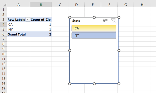
Working with multiple Excel sheets is common for many spreadsheet users. However, managing and consolidating data across worksheets and workbooks can be tedious and time-consuming without the right techniques. Master these tricks to merge and manipulate Excel sheets like an expert.

View Sheets Side-by-Side

Rather than constantly switching between tabs, view multiple sheets side-by-side in the same window. Go to the View tab and select “New Window” to open a second window displaying your workbook. You can tile or cascade sheets and easily refer to data across windows.

Link Sheets with 3D Formulas

Build 3D formulas to analyze data across multiple sheets. Start a formula as usual and add the sheet name followed by an exclamation point before the cell reference, like =Sheet2!A1. This pulls data from Sheet2 into your formula on the active sheet for seamless cross-referencing.

Consolidate Data with PivotTables

Easily combine, summarize, and report on data from separate sheets with PivotTables. When creating a PivotTable, check the box for “Multiple Consolidation Ranges” and add all the source sheets. The PivotTable will automatically pull and consolidate the data for flexible reporting.

Merge Tables with Power Query

For a more permanent data merge, use Power Query to combine tables from different sheets into a single master table. Load the sheets you want to merge, select the tables, go to the Transform tab, and click “Merge Tables”. Power Query will append the rows together into one unified dataset.

Link Cells Across Sheets

Rather than retyping the same data in multiple sheets, you can link cells and ranges across sheets to maintain consistency. Type “=” in a cell, then click the sheet tab and select the cell to link. The data will remain synced as it’s updated.

With these tips, you can masterfully merge, consolidate, and manage data across all your Excel worksheets. Want to take your Excel skills even further? Check out our upcoming workshop!

And, we’ve got you covered with an entire library of solutions that will empower you to work smarter!

Data Cleansing in Excel: Streamlining Your Analysis Workflow

August 4, 2023 by Madeleine Moucheron

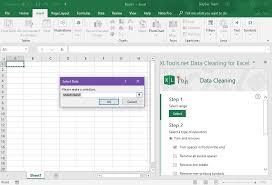
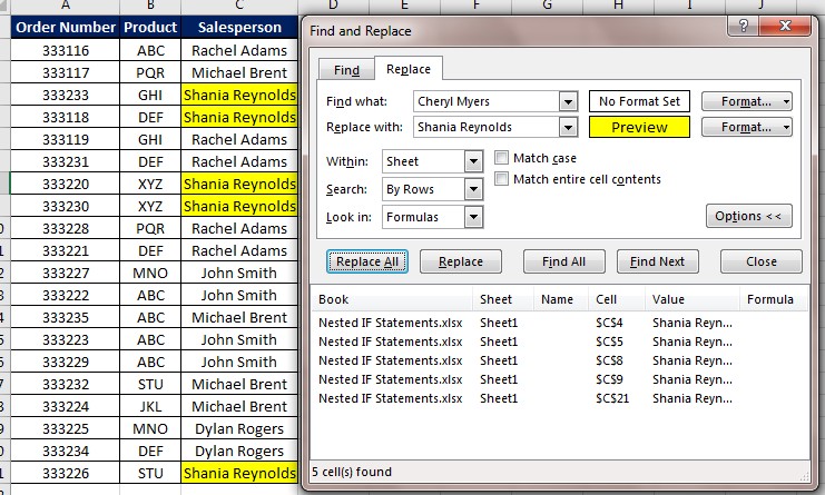
Data is the foundation of any analysis, decision-making process, or business strategy. However, raw data seldom comes perfectly organized and error-free. That’s where data cleaning and preparation play a crucial role in transforming messy data into valuable insights. Excel, being one of the most widely used tools for data management, offers a host of powerful features and best practices to ensure accuracy and reliability.

  1. Identify and Handle Missing Data: Missing data is a common issue that can distort the analysis. Excel provides tools like filtering and conditional formatting to identify and handle missing values. One can choose to either remove incomplete records or use imputation techniques to estimate the missing data.
  2. Remove Duplicate Records: Duplicates can introduce bias and affect the integrity of the analysis. Excel’s “Remove Duplicates” feature allows users to quickly identify and eliminate duplicate rows, ensuring the data remains clean and accurate.
  3. Data Validation: Implementing data validation rules can prevent erroneous data entry. Excel’s data validation feature allows setting criteria for data cells, ensuring users enter only valid and relevant information.
  4. Proper Formatting and Consistency: Inconsistent formatting can lead to data interpretation issues. Excel enables users to format cells consistently and convert data types as required. This ensures that numerical data is treated as numbers, dates as dates, and text as text.
  5. Handling Outliers: Outliers can significantly impact statistical analysis. Excel’s functions such as “IF,” “COUNTIF,” and “AVERAGEIF” help identify and deal with outliers effectively, preserving the accuracy of the data.
  6. Splitting and Combining Data: Sometimes, data may be combined in a single cell, leading to complications during analysis. Excel offers functions like “Text to Columns” and “Concatenate” to split and combine data elements, respectively, ensuring data is organized correctly.
  7. Remove Unnecessary Characters and Spaces: Excel’s “TRIM” function is useful for removing extra spaces, while “SUBSTITUTE” can help eliminate unnecessary characters or symbols from the data.
  8. Date and Time Formatting: When dealing with date and time data, Excel allows users to format these values consistently and manipulate them using various functions for better analysis.
  9. Protecting Clean Data: After cleaning and preparing the data, it’s essential to protect it from accidental changes. Excel offers password protection and sheet locking to safeguard the accuracy of the cleaned dataset.
  10. Document Data Cleaning Steps: Finally, it’s vital to document the data cleaning steps taken in a separate sheet or cell comments. This documentation ensures transparency and enables reproducibility in case of future analyses or audits.

In conclusion, data cleaning and preparation are vital steps to ensure accurate and reliable analysis in Excel. By following these best practices, users can transform raw and messy data into valuable insights that drive informed decision-making and business success. Remember, investing time in data cleaning ultimately saves time and resources in the long run, while ensuring the integrity and accuracy of your data-driven endeavors.

If you want to take your tackle Excel’s basics and beyond, check out our workshop.

And, we’ve got you covered with an entire library of solutions that will empower you to work smarter!

VLOOKUP, HLOOKUP, and XLOOKUP Formulas Part 2: HLOOKUP Formula

April 21, 2023 by Madeleine Moucheron

HLOOKUP is a function that Excel users can key in to look up and retrieve data from a specific row in a table. This function searches for values in the table’s first row, then returns a value in the same column from that row if the listed conditions are met.

Read on to discover the unique characteristics of the HLOOKUP function.

HLOOKUP

In the HLOOKUP function, the H stands for horizontal, so this function performs horizontal searches from left to right.

The HLOOKUP Function looks like this: =HLOOKUP(lookup_value, table_array, row_index_num, [range_lookup])

The components of the function have the following significance:

  • lookup_value: Like the other lookup functions, this segment identifies the piece of information you want to find
  • table_array: the table you want to search to find the specific piece of information
  • row_index_num: the row number from the table_array segment that will produce the matching value
  • range_lookup: the value that determines whether you want the function to locate an exact match or an approximate match

We hope this helps you feel comfortable using the HLOOKUP formula in Excel.

For a detailed demonstration from an expert, with exercises, and the most common questions answered, check out our workshop: Mastering Excel Lookup Functions: What Every User Should Know.

If you’d like to learn additional Excel formulas that can make your job easier, quicker, and more accurate, we’ve got you covered!

Like Learn Excel Now? Follow us on social media and share our content with your networks!

10 Reasons to Use Excel Tables

March 10, 2023 by Madeleine Moucheron

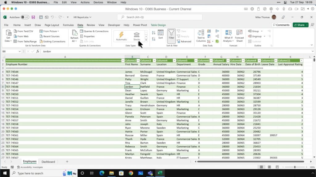
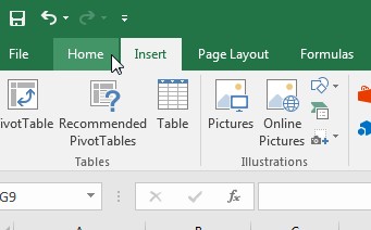
Excel tables come with a variety of features that make data recording and management a breeze. Instead of handling your data processes manually, save time and take steps to ensure accuracy by using Excel to your advantage.

Read on to learn about 10 beneficial features that make Excel worth a try.

Excel is designed to simplify data collection and analysis, and in doing so, this tool saves time, ensures accuracy, and provides valuable data insights. Take your tables to the next level by learning how to harness each of the features included in Excel.

10 Reasons to Use Excel Tables

1. Instant Formatting: Formatting an Excel table is incredibly easy if you use the “Format as Table” option or scroll through the various “Design” tabs. Simply select the format option you want and apply it to your entire table, or a portion of it (if desired).

2. Instant Filter Buttons: Using a feature known as “Slicers,” you can create quick, easy filters that allow you to organize your various datasets.

3. Instant Freeze: By selecting a cell below the rows you want to freeze, or to the right of columns you want to freeze, selecting the “Freeze Panes” option from the View tab instantly freezes your selection.

4. Instant Defined Area: Under the Formulas tab, the “Create from Selection” tab enables you to define specific areas within your table.

5. Easy Management of Data Ranges: If you select a specific design or format for your entire table (or sections of it), the selections remain as you go. This way, you don’t have to manually change every cell, row, or column.

6. Easy Insert/Delete Table Rows and Columns: You can right-click on any cell in your table to delete it, or you can choose to insert columns and rows above, below, or beside the cell.

7. Total Row On: Under the Tools tab and the Design subtab, clicking Total Row will insert a Total Row at the bottom of your table. Choose the column you want a total for, then choose the formula you need. The total will populate in the new row.

8. Auto Names and Fills: Clicking the Auto Fill Options tab presents you with a selection of auto-fills you can use. From there, select the cells you want to use to begin automatically filling data. If you’re numbering the cells, place 1 and 2 in the first two cells, then drag the fill handle to select the cells you want to fill. Apply the fill option you want.

9. Summarize with PivotTable: PivotTable is a useful feature that summarizes large datasets and provides viewers with analysis and valuable insights they can use to simplify data reviews.

10. Easy Convert to Range: Converting a list is easy with the “Convert to Range” option, which can be accessed through the Tools tab, then the Design subtab. 

Excel is designed to simplify data collection and analysis, and in doing so, this tool saves time, ensures accuracy, and provides valuable data insights. Take your tables to the next level by learning how to harness each of the features included in Excel.

For a even more excel essential from an expert, with exercises, and the most common questions answered, check out our workshop: Microsoft Excel: The Basics & Beyond for Today’s Top Professionals.

If you’d like to learn additional Excel formulas that can make your job easier, quicker, and more accurate, we’ve got you covered!

Like Learn Excel Now? Follow us on social media and share our content with your networks!


Reviewing Formulas and Functions Part 2: AVERAGE in Excel

February 23, 2023 by Madeleine Moucheron

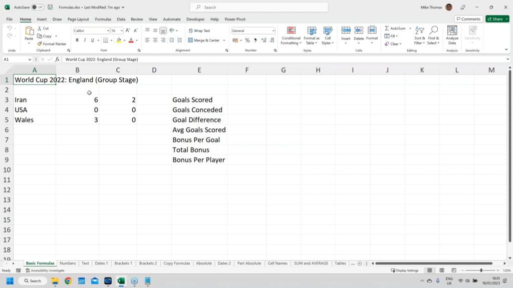
Learning a selection of Excel formulas can take your reports to the next level. Mastering a few tips and tricks can not only save time for working professionals but using Excel formulas can help double-check the values listed on a spreadsheet. To simplify your work and make sure you’re presenting accurate data, take a look at how to use the AVERAGE formula.

AVERAGE in Excel

The AVERAGE function is used to determine the average value or number in a list of numbers. It effectively finds the midpoint of a number sequence. 

Using the AVERAGE Formula

To determine the average of a list of numbers in an Excel spreadsheet, use the following formula:

  • =AVERAGE(C4:C9)

You can also find the average of several number sequences by separating them with commas.

  • =AVERAGE(C4:C9, B5:B7)

We at Learn Excel Now hope you feel comfortable creating using the SUM function in Excel. Next week, we’ll wrap up the series with COUNT function in Excel so stay tuned!

Like Learn Excel Now? Follow us on social media and share our content with your networks!

Excel Data Validation: An Introduction

December 7, 2016 by Tyrone Pernsley

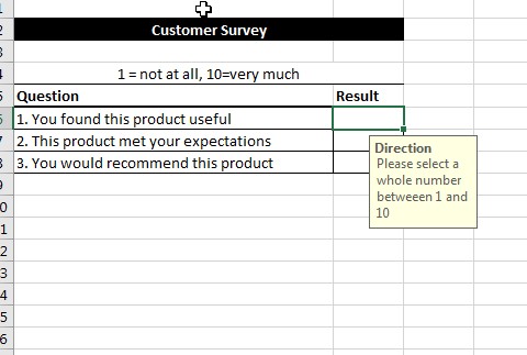
Excel data validation allows you to set specific criteria for the type of data that can be entered into a cell or group of cells. In addition to creating that criteria, you can write a brief message on what can be entered into the cell and error message when the wrong information is entered.

In today’s example, we will use the following customer survey as our example:

data-validation-image-1

Here, we need to set data validation so only whole numbers between 1 and 10 can be entered. To do this, we will:

  • Go to the Data tab
  • Go to Data Validation
  • Open the Data Validation Dialogue box
  • On the Settings tab, set the range (whole numbers between 1 and 10)
  • On the Input message, enter our unique message
  • On the Error Alert tab, enter your custom error message

Once you hit okay, the rules will apply. Here is a demonstration in Excel:

data-validation

As you can see, the only numbers that can be entered are whole numbers between 1 and 10. There are a variety of reasons to use Excel data validation and it depends on the situation and problem you’re trying to solve.

We here at Learn Excel Now hope you found today’s lesson on Excel data validation useful.

Like Learn Excel Now? Follow us on social media and share our content with your networks! And don’t forget to sign up for the Newsletter

Kevin – Learn Excel Now

Excel Essentials: Running Spell Check in Excel

October 5, 2016 by Tyrone Pernsley

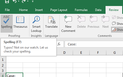
Excel offers many built-in tools to help you perfect your spreadsheets. Some of these tools, however, need to be activated rather than running automatically. Today, we explore one such tool: running spell check in Excel.

When most people think Excel, the first thing that comes to mind is numbers. But text is often required in Excel to put those numbers into context. This is especially true on any type of report where you might need to add background information, explain your thought process, or just explain where the numbers on the page came from. Even something as simple as column headings, or a client name will require written text.

When submitting reports, you want the spreadsheet to be as accurate as possible and look good. Misspellings and typos simply won’t do. But unlike many Microsoft programs (Word, Outlook, PowerPoint, etc.), Excel doesn’t automatically spell check, giving you those convenient squiggly, red lines when something is wrong. This can make it extremely difficult to catch little errors.

Let’s say you had the following spreadsheet:

excel-spell-check-image-1

Maybe you can recognize all of the typos right away, maybe you can only see a few. The only way to be sure you caught all of the misspelled words is to run Spell Check:

excel-spell-check-gif

As you can see in the above spreadsheet, all of the misspelled words were fixed:

  1. “projcet” was changed to “project”
  2. “prdoucts” was changed to “products”
  3. “incrase” was changed to “increase”
  4. “esitmated” was changed to “estimated”
  5. “retruns” was changed to “returns”

Excel spell check is the perfect tool for verifying accuracy and correcting mistakes when it comes to text in Excel.

We at Learn Excel Now hope you feel comfortable checking the spelling in your text.

Like Learn Excel Now? Follow us on social media and share our content with your networks! And don’t forget to sign up for the Newsletter

Kevin – Learn Excel Now


Excel Essentials: Adding Images to a Spreadsheet

September 28, 2016 by Tyrone Pernsley

Excel has many tools to help you master the look and feel of your spreadsheet. One feature it offers is the ability to add images to your spreadsheet. It can be an object from clip art, an original photo, downloaded images – as long as it’s in an image file, you can add it to Excel.

Let’s say you were putting together a sales report to send out to potential vendors. You are working with the following spreadsheet:

image-1

Now, your boss tells you he wants to add the company logo to the spreadsheet to give it a more polished and professional look. This is the process for adding the company logo:

adding-images-to-a-spreadsheet

  • Step 1: Prep your spreadsheet for the added image
  • Step 2: Go to the “Insert Ribbon”
  • Step 3: Click on the icon for ‘Pictures’
  • Step 4: Select the image you want to use in the dialogue box
  • Step 5: Click OK
  • Step 6: Using the Drag options on the image, resize to preferred size
  • Step 7: Double check to make sure it looks good.

You are now done with adding the company logo. Adding images to your spreadsheets can add value, relevance or just make them more fun.

We at Learn Excel Now hope you now feel confident adding images to Excel and formatting them to make your spreadsheets look great.

Like Learn Excel Now? Follow us on social media and share our content with your networks! And don’t forget to sign up for the Newsletter

Kevin – Learn Excel Now

Excel Find & Replace: Building Fundamental Skills

September 7, 2016 by Tyrone Pernsley

Find and Replace Featured Image (2)Excel contains tons of built-in tools designed to help you do what you need to. This week we are talking about one of those tools, the robust Find and Replace tool. In the following guide, we will explore how to use this tool and situations where it could be needed.

Simple Find Function

To find something in Excel, you use the simple Find function you use in any other program, Ctrl F. This opens the Find dialogue box where you can enter the text of what you’re looking for. However, Excel contains other built-in options in the dialogue box that allow you to go beyond the simple find function. We will explore those options later in this guide.

The important thing to remember is the keyboard combination Ctrl F at the same time.

Find Dialogue box

Replace What You Found

As you can see in the above image, the dialogue box contains a tab that states “Replace.” Once you found the items you are looking for, you can easily replace them using this tool.

Let’s say you had the following spreadsheet listing what clients each salesperson represents:

Replace Image 1

Now, your boss informs you that Cheryl Myers will be leaving the company. A new employee, Shania Reynolds, will be taking over her sales. Manually replacing Cheryl’s name with Shania’s in each instance would be tedious and time consuming (especially in larger worksheets!). Plus you could always run the risk of missing a location. Luckily, you can use the Replace tool to quickly find and replace all instances in a few clicks:

  • Use the Ctrl F keyboard combination to open the dialogue box
  • On the Find tab, enter the data you want (Cheryl Myers in this instance)
  • Click on Find All to ensure all instances are located
  • Then click on the Replace Tab
  • On the “Replace With” line, enter the new data (Shania Reynolds in this instance)
  • Click on Replace All

As you can see in the following GIF demonstrating these steps, all instances of Cheryl Myers are replaced with Shania Reynolds

Find and Replace GIF 1

Special Formatting for Replacing

The options for Excel’s Find and Replace tool don’t stop there. You can also use the tool to format specific cells. Let’s say your boss wanted you to highlight the new employee’s areas for quick reference. Again, you can do this manually, but it would be a waste of time. Instead, you could:

  • Use Ctrl F to open the dialogue box
  • Enter the data you want to find (Shania Reynolds)
  • Click Find All
  • On the Replace Tab, open the Options dialogue
  • Select Format on the “Replace With” line
  • Go to the tab that says “Fill”
  • Select the color you wish to use for highlighting (yellow)
  • Click “Replace All”

As you can see in the following GIF, the name is still in the cells, but it has been highlighted yellow.

Find and replace GIF 2

We at Learn Excel Now hope you now feel comfortable using the Find and Replace tool. This tool contains other formatting options to change the cells containing data you found. Using the tool is a matter of personal need, but there are many situations where it comes in handy.

Like Learn Excel Now? Follow us on social media and share our content with your networks! And don’t forget to sign up for the Newsletter.

Kevin – Learn Excel Now

How to Calculate a Subtotal In Excel Using the Filter

July 20, 2016 by Tyrone Pernsley

Excel has many ways to calculate data. If you know the right formulas and functions, you can find out just about anything you want to know about your data. Today’s lesson is on using the subtotal formula to find various totals based on the filter option in Excel.

Imagine you are running sales numbers using the following the spreadsheet:

Calculating Subtotals Image 1

If you remember from last week’s blog post on Sorting and Filtering data, we have gone ahead and added the filter. Now, if you wanted to find the sales total, you can use the following formula:

=sum(range)

This is the standard way to find a total. But, as you can see, once you use this formula and change the anything from the filtered drop-down menu, the sales total doesn’t change with it:

Calculating Subtotals Gif 1

So, how do you get the total to change with changes you make on the filter? This is where you will use the Subtotal formula. The Subtotal formula is:

=subtotal(function_number, ref1…)

Note: You need to select which function you want the subtotal to use. For finding sums, we use function 9-Sum. As you can see from the following menu, there are multiple functions to choose from:

Subtotal Menu Options

Once the function is selected it’s time to enter the range. For the spreadsheet example, we are looking for subtotals on the Sales column, Column D. So, the final formula looks like this:

=subtotal(9,D2:D21)

When you first enter this formula in cell D22, it gives you the total amount, the same as when you enter the Sum formula. However, watch what happens when you change the options using the Filter drop-down:

How to Calculate a Subtotal In Excel Using the Filter

As you can see, the Subtotal formula lets you find totals by Salesperson, Client, Product, etc. quickly and easily. And the total changes with the information you select.

We here at Learn Excel Now hope you found today’s tip on how to calculate a subtotal useful.

Like Learn Excel Now? Follow us on social media and share our content with your networks! And don’t forget to sign up for the Newsletter

Kevin – Learn Excel Now

  • 1
  • 2
  • 3
  • Next Page »
All Access Subscription
Our 1-year all-access subscription provides step-by-step guidance for mastering Microsoft Office applications, with workshops, exercises and quick reference eGuides. It's perfect for anyone that needs to brush up on certain skills or even folks who need to learn the programs - from a beginner’s level.
Excel Foundations
Take the fear out of Excel with this 20 module self-paced training course. You will cover the most essential topics to develop a solid foundation of Excel or a lifetime of mastery.

Learn Excel Now helps you conquer the fear of Excel. By providing self-paced and instructor-led training and free strategies and guides, we leave no Excel mystery unsolved.

  • Home
  • Training
  • All-Access
  • Excel Foundations
  • Resources

Connect with Us

  • Facebook
  • Linkedin

Contact

Learn Excel Now
questions@learnexcelnow.com
1-484-259-7664 or 1-800-964-6033
660 American Ave
Suite 203
King of Prussia, PA 19406

Microsoft® Office Excel® is a registered trademark of the Microsoft Corporation in the United States and other countries. All rights reserved.

Copyright © 2023 ­Learn Excel Now

Terms of Service

Privacy Policy

Copyright © 2023 · News Pro Theme on Genesis Framework · WordPress · Log in

WELCOME BACK!

Enter your username and password below to log in

Forget Your Username or Password?

Reset Password

Lost your password? Please enter your username or email address. You will receive a link to create a new password via email.

Log In