Excel Find & Replace: Building Fundamental Skills

September 7, 2016 by Tyrone Pernsley

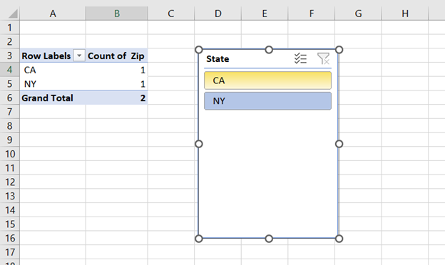
Excel contains tons of built-in tools designed to help you do what you need to. This week we are talking about one of those tools, the robust Find and Replace tool. In the following guide, we will explore how to use this tool and situations where it could be needed.

Simple Find Function

To find something in Excel, you use the simple Find function you use in any other program, Ctrl F. This opens the Find dialogue box where you can enter the text of what you’re looking for. However, Excel contains other built-in options in the dialogue box that allow you to go beyond the simple find function. We will explore those options later in this guide.

The important thing to remember is the keyboard combination Ctrl F at the same time.

Replace What You Found

As you can see in the above image, the dialogue box contains a tab that states “Replace.” Once you found the items you are looking for, you can easily replace them using this tool.

Let’s say you had the following spreadsheet listing what clients each salesperson represents:

Now, your boss informs you that Cheryl Myers will be leaving the company. A new employee, Shania Reynolds, will be taking over her sales. Manually replacing Cheryl’s name with Shania’s in each instance would be tedious and time consuming (especially in larger worksheets!). Plus you could always run the risk of missing a location. Luckily, you can use the Replace tool to quickly find and replace all instances in a few clicks:

Use the Ctrl F keyboard combination to open the dialogue box
On the Find tab, enter the data you want (Cheryl Myers in this instance)
Click on Find All to ensure all instances are located
Then click on the Replace Tab
On the “Replace With” line, enter the new data (Shania Reynolds in this instance)
Click on Replace All

As you can see in the following GIF demonstrating these steps, all instances of Cheryl Myers are replaced with Shania Reynolds

Special Formatting for Replacing

The options for Excel’s Find and Replace tool don’t stop there. You can also use the tool to format specific cells. Let’s say your boss wanted you to highlight the new employee’s areas for quick reference. Again, you can do this manually, but it would be a waste of time. Instead, you could:

Use Ctrl F to open the dialogue box
Enter the data you want to find (Shania Reynolds)
Click Find All
On the Replace Tab, open the Options dialogue
Select Format on the “Replace With” line
Go to the tab that says “Fill”
Select the color you wish to use for highlighting (yellow)
Click “Replace All”

As you can see in the following GIF, the name is still in the cells, but it has been highlighted yellow.

We at Learn Excel Now hope you now feel comfortable using the Find and Replace tool. This tool contains other formatting options to change the cells containing data you found. Using the tool is a matter of personal need, but there are many situations where it comes in handy.

Like Learn Excel Now? Follow us on social media and share our content with your networks! And don’t forget to sign up for the Newsletter.

Kevin – Learn Excel Now

Excel Basics: Adding, Editing & Formatting Comments

August 31, 2016 by Tyrone Pernsley

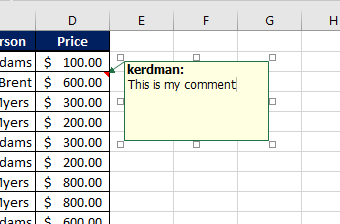
In Excel, you can add a comment to any cell. This could be a note to yourself, a reminder, a correction, a question – anything that is useful. Using Excel comments is particularly useful for workbooks that are used to share information and to collaborate on projects. At times though, you might want to go beyond the basic comment format and give your comments more character.

First, let’s explore the basic comment. To add a comment, you will:

Right click on the cell you want to comment on
On the menu, select comment
Enter your comment in the comment box that opens

Once you click out of it the comment will be part of the cell

Any cell with a comment has a small, red triangle in the upper right hand corner.

Now if anyone opens this workbook they will be able to view what you wrote. This is the basic comment format:

Formatting Comments

As with most things in Excel, you can do more with your comment than what the default format has to offer. To open editing for your comment, you will:

Either create a new comment or click on Edit Comment in the menu
Once the comment box is open, right click on outer edge of the box
Select Format Comment

Once you’ve open the format comment dialogue box, you have several options:

From there, you can make whatever changes you see fit:

Why Change Excel Comment Formatting?

There could be several reasons to change the formatting for comments:

Personal preference
Color coding types of comments
Adding urgency or priority to comments
And many others

We here at Learn Excel Now hope you found this week’s tip on Excel comments useful.

Like Learn Excel Now? Follow us on social media and share our content with your networks! And don’t forget to sign up for the Newsletter.

Kevin – Learn Excel Now

Excel Formatting Essentials: Hiding Extra Rows & Columns

August 24, 2016 by Tyrone Pernsley

Today’s Excel blog post comes directly from a Learn Excel Now customer who was having trouble formatting her spreadsheet. She wanted to hide the extra rows and columns of the spreadsheet grid after creating a chart.

Here is what she wrote to Learn Excel Now:

“I produce weekly reports for my boss. He likes them to be in a 3D Pie Chart. But I can never seem to format it correctly. He showed me the report my coworker Carol sends him. It’s just a single chart – there is no spreadsheet behind it! It looks so clean and neat, like a single image. I want to be able to do that.”

And she can. For today’s example we will take the following spreadsheet and create a chart. Then we will format that chart so that it is the single image in the worksheet.

To create the chart:

Highlight the group of cells you want to chart
Go to the Insert tab on the home ribbon
Select the type of chart you want to use (3D Pie Chart in this case)

To make the chart the single image on the worksheet:

Expand the chart to cover the underlying data in the spreadsheet
Click on the first column visible to the right of the chart
Enter the keyboard shortcut Ctrl+Shift+à (right arrow key) to go to the last column
Open the right click menu and select Hide
Click on the first row visible underneath the chart
Enter the keyboard shortcut Ctrl+Shift+Down Arrow Key to go to the last row
Open the right click menu and select Hide

You have now hidden all of the rows and columns in the spreadsheet, leaving the chart as the lone visible image on the worksheet. Here is a Gif showing what to do:

Using the keyboard shortcuts to go to the last row and column can come in handy in many situations. Anytime you want to make the spreadsheet a close off image, you can hide those rows and columns.

We here at Learn Excel Now hope you feel comfortable using this convenient formatting tool.

Like Learn Excel Now? Follow us on social media and share our content with your networks! And don’t forget to sign up for the Newsletter.

Kevin – Learn Excel Now

Removing Duplicates in Excel: Quick How-to Guide

June 22, 2016 by Tyrone Pernsley

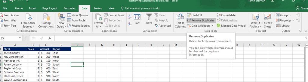
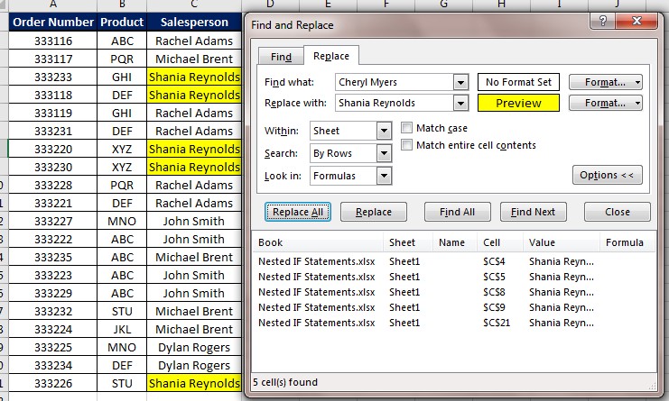
This Excel tip from Learn Excel Now is on removing duplicates in Excel. The request is directly from a Learn Excel Now fan who asked us how to quickly remove duplicates. She told us:

“I pulled a list of all company sales from our database. It exported in Excel. The list is all of our sales, but many of our clients buy multiple products several times through the year. Yesterday, my boss asked me ‘how many unique clients have purchased in the last month?’ Those figures aren’t available because we’ve always only counted total sales. I started counting the individual companies 1-by-1, but there are so many of them. I know there has to be a way to remove the duplicates so I can see each company listed only once. Can you help me?”

So, this post was designed for one of our fans – let’s call her Rachel – and anyone else who wants to know about removing duplicates in Excel.

The following table contains multiple cases of duplicates. Similar to Rachel’s request, they are the names of companies in a sales document.

Now, let’s get in there and remove those duplicates! Here’s how you do it:

Highlight the column(s) or row(s) containing the duplicate values you want to remove
Go to the ‘Data’ Tab on the Excel Ribbon
Find the “Remove Duplicates” tool and click it
Verify the table range on the dialogue box OR select the correct range on the dialogue box

If there are more values in the table but you want to stick to a column or row, select “Use Current Selection

Excel will automatically remove all duplicates. Now you and review and count the total unique values within the range.

We here at Learn Excel Now hope you now feel confident in removing duplicates in Excel. This useful tool is great for running quick analyses, finding unique values and cleaning up datasets for other functions or formatting.

Like Learn Excel Now? Sign up for the e-newsletter to receive weekly Excel tips and special offers just for you!

And don’t forget to follow us on social media and share our Excel tips with your networks!

Kevin – Learn Excel Now

Creating Excel Tables: Quick Tip to Get Up-to-Speed

June 15, 2016 by Tyrone Pernsley

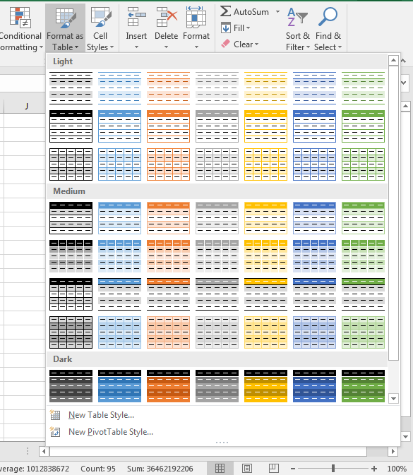
Excel provides you with many preset formatting options that you simply need to click to activate. One of the most common and most useful is to set your data as a table. There are many advantages to organizing your data in a table. It makes it easier to sort and filter important data, find totals automatically and create charts and graphs.

Setting your data as a table is fairly easy. First, you take your basic dataset:

And then you apply the table setting:

As you can see from the above Gif, there are many table styles to choose from:

This gives you the power to customize your Excel table to your preference.

Pro tip: you can add more customization to your formatting by using the Cell Styles tool to add colors, text formatting and other elements to make your table pop:

Once you have your table formatted, you can us the dropdown menu to quickly filter information:

You also have the ability organize your dataset in a variety of ways.

We here at Learn Excel Now hope you enjoyed this week’s quick tip on Excel Tables.

Like Learn Excel Now? Follow our social media pages and share out content with your networks!

Kevin – Learn Excel Now

Excel Merge & Center – What It is & How to Use It

June 8, 2016 by Tyrone Pernsley

The following article shows you how to use the Excel Merge & Center tool.

The spreadsheet software of Microsoft Excel is best known for crunching numbers. This remains the primary reason people use Excel. But often times, you need text to accompany those numbers to make sense of what the numbers mean. Whether it’s column headings, naming the worksheet itself, itemization or important notes, adding text to Excel is a vital component of making your Excel spreadsheets be professionally viable.

Sometimes adding text can create formatting issues. Fortunately, Excel provides formatting options to make your spreadsheet accommodate text without compromising the number formatting. One such tool is the Merge & Center tool. This is perfect for text that runs over multiple cells. Without changing the Excel width or height of the individual cells in a column or row, you can merge all the cells together. The text will also automatically expand.

Let’s take the following spreadsheet as an example. The name of the spreadsheet has been added to the spreadsheet:

Notice how the text for the name of the spreadsheet runs from A1 to C1. The table, however, is already formatted so that the columns are the right width for the Column Headings. Adjusting column width for the name of the spreadsheet throws everything off:

This is where the Excel Merge & Center tool comes into play. The following Gif will show you how to use the tool:

Now, as you can see above, the text for the spreadsheet heading runs the width of the table. But none of the columns or rows containing table data had to adjust. This is now a fixed heading.

From there, you can format the color, text size, etc. to get the heading exactly how you want it.

We here at Learn Excel Now hope you now feel comfortable using the Excel Merge & Center option.

Like Learn Excel Now? Follow us on social media and sign up for the newsletter!

Don’t forget to share our tips with your friends and colleagues!

Kevin, Learn Excel Now.

Excel Number Formatting Special: Phone Numbers

June 1, 2016 by Tyrone Pernsley

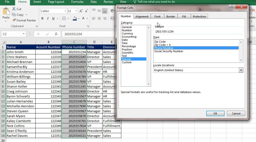
Excel gives you the power to format your numbers in a ton of different ways. Today’s post is focusing on one specific, special format: phone numbers. We here at Learn Excel Now are continuously surprised by the number of people who say they didn’t know this was an Excel Feature. So, to help make sure everyone using Excel knows how to create special number formatting, we created the following quick tip.

Let’s say you exported a customer list from your database in an Excel file. There is no formatting in the new file and looks a bit like this:

So, the first thing you do is automatically expand the columns and possibly add a bit of color to the spreadsheet so it looks like this:

Now, in order to change the numbers to phone numbers, you will need to:

Highlight the cells containing the data you want to format
Click on the dropdown button on the Number tab of the Home Ribbon

On the Format Cells dialogue box that opens, click Special and then Phone Number

Once you click Okay, the cells automatically format as phone numbers:

You will see there are other options on the Special formatting:

Zip Code
Zip Code + 4
Phone Number
Social Security

Any of these options will allow you to format the numbers in an easy to read way.

We hope you enjoyed this week’s quick tip on formatting Excel for numbers.

Like Learn Excel Now? Sign up for our newsletter to stay up-to-date on all things Excel?

And don’t forget to follow us on social media and share our Excel tips with your social networks!

Kevin – Learn Excel Now

Setting Dates in Excel: Repeating, Consecutive & Custom

May 25, 2016 by Tyrone Pernsley

Ever been frustrated by repeatedly typing in dates in Excel? You know there is a way to make dates appear in order or repeat but you do not have time to test out how to do it. If this is a daily problem for you than you are in the right place! Today we will show you how to repeat, change or make a pattern of dates in an excel spreadsheet with a few clicks!

To create a spreadsheet continuous dates:

First enter the date out in the desired cell that will begin your sequence
Click on the cell that contains your first date and hold down the bottom right of the cell and drag downward/rightward.

You will notice that the proceeding dates appear once you have released your click! A full calendar, at the click of a button!

To create a spreadsheet with a repeating date:

Enter the date out in the desired cell that will begin your sequence
in the next cell below/to the right enter =cell that contains the date to be repeated. (If your date is in A1, you would enter =A1 in the proceeding cell).
After this is done, hit enter, click the cell and drag the cell down from the bottom right.
Notice that this allows for the desired date to be repeated as many times as you like!

Say you want to have the date repeated twice before proceeding to the next date. To create a pattern that you would like your dates to follow, first enter your desired date in a cell. In the next cell, enter =A1 (or whatever the first cell is) and =A2+1 in the next and =A3 in the next. Like this:

A1- 6/03/2015

A2 – =A1
A3 – =A2 + 1
A4 – =A3

Now select cells A3 and A4, click the bottom right of the selection and drag down to your desired range. You will see that now you have the each date repeated twice! Pretty cool right!? Test out some other patterns and try different things out now that you understand this concept!

Follow the GIF above if you are having any issues! It is a good visual for a difficult concept like this!

We hope you found todays quick and easy Excel lesson beneficial. Don’t forget to follow ups on Social Media and subscribe to the blog to get convenient, quick tips like this, and other great Excel training tips so that you can take the fear out of Excel.

Like Learn Excel Now? Sign up for the newsletter!

Kevin, Learn Excel Now

Changing the Alignment of Data in an Excel Cell

May 4, 2016 by Tyrone Pernsley

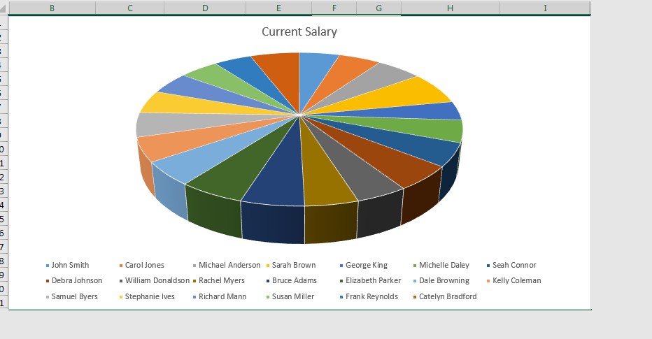
Making an excel spreadsheet look “pretty” is not as daunting as people make it seem. Many people in the workforce will shy away from tinkering with an excel spreadsheet’s layout because they have a fear of making it worse or deleting an important item. Today our goal is to crush the fear of alignment of data in an excel cell!

Have you ever had numbers in the cells adjacent to a text wrapped group of cells? With a giant cell, numbers do not always fill the up the empty space which makes the spreadsheet look awkward. Here is how to fix that issue in the matter of seconds.

There are two ways to do this. The first way is to use the “Alignment” in the general toolbar on top of your excel spreadsheet. It looks like this.

First, highlight the cell or cells that you desire to have their contents aligned. Go up to the alignment toolbar and chose either the left, center, or right alignment. After your desired horizontal alignment has been chosen, chose your vertical alignment (top, center, or bottom). In seconds you can transform how your spreadsheet to look clean and neat!

The second way to go about this would be to right-click the cell or selection of cells that you would like to change the alignment for. Select “Format Cells” at the bottom of the menu and click the “Alignment” tab. From there you can select the type of Horizontal and Vertical alignments with a drop down menu. You can also use the “Orientation” area to rotate the data of your cell if you really want to get crazy! Once you are finished changing your settings, click OK.

Check out the demonstration below to get a better understanding of the two ways to change the alignment of data in an excel cell.

Like Learn Excel Now? Sign up for the newsletter above! And don’t forget to connect with us on social media and share your favorite Excel tips with your networks!

-Kevin, Learn Excel Now

Wrapping Text in Excel: Formatting Foundations

April 13, 2016 by Tyrone Pernsley

Have you ever had so much data in one cell that that it spills over to the next cell or just disappears? And you don’t want to expand cells because it throws off data presentation in other cells? If you would like to solve this issue, then we are here to help you with wrapping text in Excel!

Like many excel features, there are short and long ways of executing the task. So we will show you both!

First, a quick way to wrap text for every cell is by going to the “alignment” section of your home toolbar and clicking the icon in the first row, 4^th column.

If you hover over this icon with your mouse you will see it says, “Wrap text”. Click this icon and bam!, now all data will automatically be wrapped to fit the column width

The second way to do this is to first, highlight your desired cell or group of cells. Right click, select “format cells”, chose the “alignment” tab, check off “wrap text”, and click Ok.

If all wrapped text is not visible, it may be because the row is set to a specific height so you may need to play around a little bit to get it to look how you want it too,

The nice part about excel is that you do not have to be afraid of getting your spreadsheet to look how you would like it too. With the text wrapping feature and your prior knowledge of adjusting rows and columns (from our previous post) you have the freedom to customize!

We hope you found today’s quick and easy Excel lesson beneficial. Don’t forget to follow ups on Social Media and subscribe to the blog to get convenient, quick tips like this, and other great Excel training tips so that you can take the fear out of Excel.

Like Learn Excel Now? Sign up for the newsletter!

-Kevin, Learn Excel Now

Excel Find & Replace: Building Fundamental Skills

Excel Basics: Adding, Editing & Formatting Comments

Excel Formatting Essentials: Hiding Extra Rows & Columns

Removing Duplicates in Excel: Quick How-to Guide

Creating Excel Tables: Quick Tip to Get Up-to-Speed

Excel Merge & Center – What It is & How to Use It

Excel Number Formatting Special: Phone Numbers

Setting Dates in Excel: Repeating, Consecutive & Custom

Changing the Alignment of Data in an Excel Cell

Wrapping Text in Excel: Formatting Foundations

Connect with Us

Contact

Connect with Us

Contact

WELCOME BACK!

Reset Password