Learn Excel Now

Conquer the Fear of Excel

  • Home
  • Training
    • Excel
    • MS Office
    • Outlook
    • PowerPoint
    • Word
    • OneDrive
    • Google
  • All-Access
  • eLearning
    • Excel Foundations
    • Micro Courses
      • Simply Excel
  • Resources
  • Login

Excel Essentials: How to Remove Duplicates in Excel – Video

April 6, 2016 by Tyrone Pernsley

How to Remove Duplicates in Excel

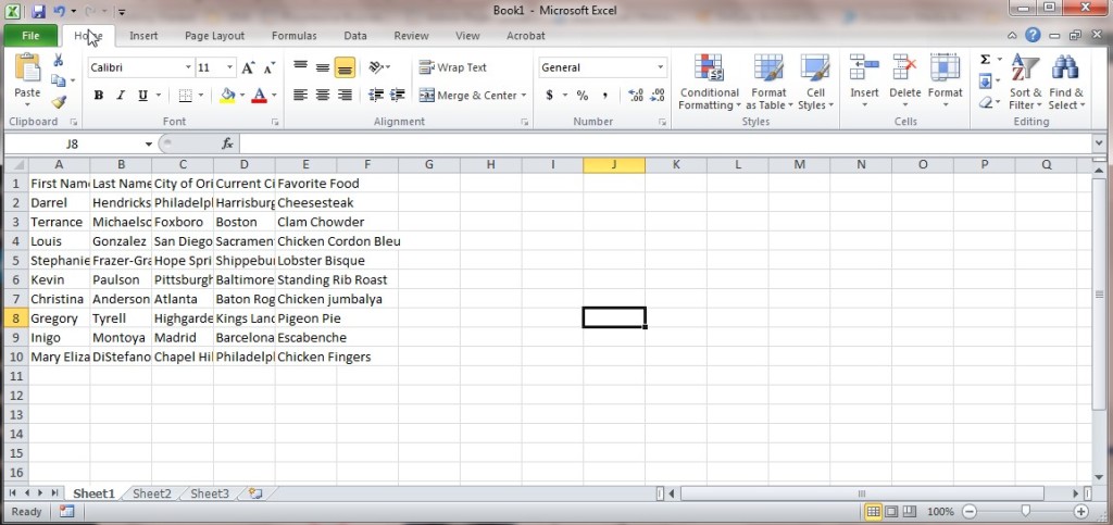
Clean, readable data makes Excel much easier to use. A common struggle is how to remove duplicates in Excel. Having too many duplicates causes inaccuracies in reporting and analyzing data. But scrolling through your data to hunt and peck duplicates is tedious and time-consuming – especially when you have hundreds of rows of data.

Even using the Find function (keyboard shortcut: Ctrl+F) can take forever. But Excel provides built-in tools to help you with this.

Please enjoy the following video on how to remove duplicates in Excel:

We here at Learn Excel Now hope you know feel confident in your ability to remove duplicates in Excel

To discover essential tips like this and so much more, please join us for:

Excel Essentials: Most Needed Skills in Today’s Workplace
Wednesday, April 13, 2016

In this live, online event, our Excel expert instructor will cover the key Excel skills you need for workplace success.

Like Learn Excel Now? Sign up for our weekly tips, announcements and offers!

Getting social with Excel – don’t forget to follow us on social media and share our content with your networks!

Kevin – Learn Excel Now

Sorting Data with Excel Pivot Tables

March 9, 2016 by Tyrone Pernsley

The Pivot Table is one of the most useful features in Excel. Sorting data with  Excel Pivot Tables allows you to examine your data from multiple points of view for better summary and analysis. You can sort data, count totals, averages, percentages, etc. In addition to giving you the ability to organize your data, Pivot Tables also makes your data more presentable.

Creating a PivotTable

Sorting Data with Excel Pivot Tables GIF 1

Once you have highlighted the data that you want in your Pivot Table report, go to the “Insert” tab and click on “Pivot Table.” You can then be able to choose to create the Pivot Table report on a new page or keep it on the same page as your data. The Pivot Table that is generated will be blank, so you have to pick which values you want and where you want them. You can arrange your data in rows or columns and include sums of different data series. To do this, you simply use the Pivot Table Field List on the right to drag and drop fields to the area where you want them to go. Your Pivot Table will then be generated and then you can sort and organize it.

PivotTable image1

Sorting Data

PivotTables can be used to organize and sort all kinds of data. Some examples include:

  • Alphabetically
  • Numerically
  • By dates and time

The options for selecting which data to look will be affected by the row and column labels in the original data set. For example, if you have a list of purchases and want to organize them by date, you can move the two column labels into the Pivot Table fields.

In the Pivot Table report, click on the drop-down arrow next to “Row Labels” or “Column Labels,” then select how you want your data to be sorted. If all of your values are words, you’ll be able to sort the data alphabetically from A to Z or from Z to A. For numeric values, you can sort it from smallest to largest or from largest to smallest. For times and dates, you can sort form oldest to newest or newest to oldest. You can also drag and move data to sort it in any way you want.

Sorting Data with Excel Pivot Tables GIF 2

Once you have your data organized into the proper fields, you can begin to summarize the findings for improved decision-making.

We here at Learn Excel Now hope you enjoyed this quick guide on sorting data with Pivot Tables. It is our desire to bring you the best advice and training available so you can effectively and efficiently use your Excel tools.

Liked this sorting data with Excel Pivot Tables quick tip? Have questions? Leave your comments below; we’d love to hear from you.

Getting Social with Excel: Spread the word and share the knowledge!

Kevin – Learn Excel Now

Basic Calculations in Excel: How to Quickly Find the Answers You Need – Video

February 17, 2016 by Tyrone Pernsley

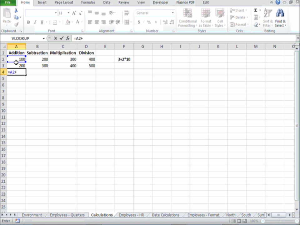
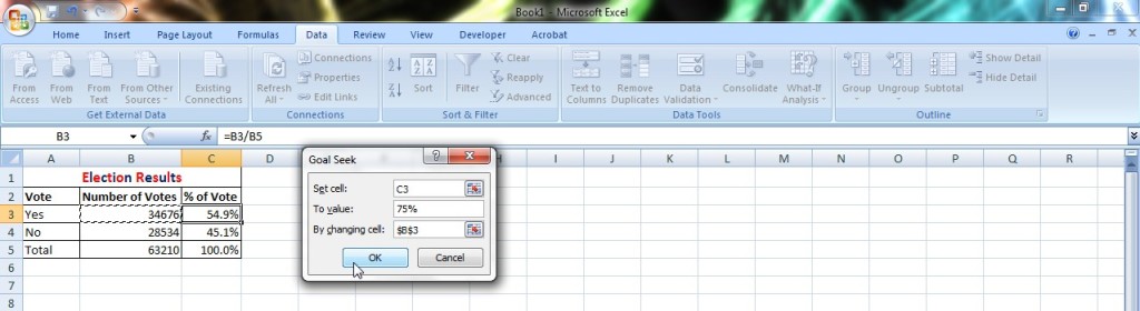
Excel has tons of formulas, functions and features to make calculations for your data. But you can also do basic calculations in Excel without using formulas. Basic calculations in Excel are great for quickly finding the results you need – be it addition, subtraction, multiplication or division – without having to enter any clunky formulas (or remembering them!)

LEN-WebVideo_BasicFormulas from Learn Excel Now on Vimeo.

Please enjoy this video on basic calculations where you will discover:

  • How to set up basic arithmetic in a cell
  • How modifying a cell in a formula will affect the answer

As you can, basic calculations in Excel are quick and easy. Here are a few keys to remember when doing basic calculations in Excel:

  • All formulas begin with the equal sign: =
  • For addition, you want to use the plus sign: +
  • For subtraction, us the minus sign, also the hyphen: –
  • For multiplication, use the asterisk (shift+8): *
  • For division, use for forward slash: /

Basic calculations in Excel are perfect when you need to find a result quickly and easily. For example, if you have two rows of sales totals and want to know their total sum, you can enter:

=(Cell1+Cell2)

Or let’s say you have a revenue and one column and cost in another want to find profit, you would enter:

=(Cell with profit total – Cell with cost total)

Another key to remember is that all cells in Excel have an alphanumeric designation; where the cell begins with the Column identify letter and ends with the Row identifying number (e.g. A1, B2, etc.)

Using the cell destination, rather than value in the cell, allows to the outcome of the formula to change if the cell value is changed.

You should be all set for using Basic calculations in Excel!

We at Learn Excel Now hope you found this week’s tip useful. Please subscribe to the newsletter to stay up-to-date with our latest tips, guides, tutorials and training!

Like Learn Excel Now? Get social with Excel! – Share this post with anyone needing Excel help on social media.

Kevin – Learn Excel Now

Converting Numbers to Percentage in Excel

February 10, 2016 by Tyrone Pernsley

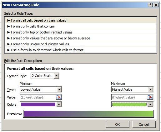
Cell formatting in Excel allows you to represent your numbers in a variety of ways: as a date, as a percentage, as currency, and with custom formatting, even phone numbers. In today’s quick tip, we are going to show you how to quickly change a number to a percentage in Excel.

After entering a number or an array of numbers into different cells, you can format them (or format the cell before the number is entered – your preference).

To convert the values to a percent:

  • Highlight the desired cells
  • Right click them
  • Click the Format Cells option
  • Click the Number category
  • Then chose the percentage tab

This will give you the option to change how many decimals points you desire to show. After you have picked your desired decimal points, click OK and bam, it is now a percentage!

Percentage in Excel GIf 1

Tip: you can also click on the lettered column heading to convert the all cells within the column to your formatting preference. This is good for spreadsheets where you will be adding values over time, so that you don’t have to keep reformatting each time.

Note:  if you apply the percentage format to existing numbers in a spreadsheet, excel multiplies the numbers by 100 to convert them to percentages. (If a cell contains 20, it will covert to 2000.00 %).

To format empty cells, follow the same procedure for formatting cells with existing values. Tip: you can also click on the lettered column heading to convert the all cells within the column to your formatting preference. This is good for spreadsheets where you will be adding values over time, so that you don’t have to keep reformatting each time.

Percentage in Excel GIF 2

As with many functions in Excel, there is another way to this as well using the Ribbon – the top toolbar in Excel.

Percentage in Excel Image 1

To change numbers to a percentage in Excel using the Ribbon, click on the Ribbon, make sure you are on the home Ribbon tab. The go to the number tab and use the dropbox to select percentage. On this tab, you can also use the decimal arrow keys to select the number of decimal places you want.

Percentage in Excel GIF 3

We hope you found today’s quick and easy lesson on converting numbers to a percentage in Excel beneficial. Don’t forget to follow ups on Social Media and subscribe to the blog to get convenient, quick tips like this, and other great Excel training tips so that you can take the fear out of Excel.

Like Learn Excel Now? Sign up for the newsletter!

-Kevin, Learn Excel Now

Getting Starting with Excel Formatting

January 20, 2016 by Tyrone Pernsley

When it come to Excel formatting, there are so many options and tools that it can be a little overwhelming trying to determine what to use and how to use it. Luckily, there are some beginning steps that can help you focus on where to begin.

Special Paste

Excel Formatting Topi Image

In the following article, we will start with some of the more basic tools and features you can use and then get into an Excel formatting macro as a suggestion on something you can do once you’re comfortable with the basic stuff.

Freezing Column Headings

When you’re working with a long excel spreadsheet, you might want to see what your column headings are so that you don’t have to keep scrolling up or make a mistake.

To make this easy, freeze the column headings. This will always keep your first row with the headings at the top of the columns regardless of how far down you scroll.

To set this, click on “View” on the tool bar, and then select “Freeze Panes.” Click on the “Freeze Top Row” option.

Excel Formatting- image 2

Quick Tips For Adjusting Columns and Rows: Your Handy Excel Formatting Cheat Sheet

  • To quickly insert a column or row, select the row or column by clicking on a corresponding cell, then click “Ctrl” and “+”
  • To quickly delete a column or row, select the row or column by clicking on a corresponding cell, then click “Ctrl” and “-”
  • Autofit makes the columns big enough to fit their contents. To do this, select the column(s) that you want to change, then click on the “Format” icon on the tool bar and select “AutoFit Column Width.”
  • Another way to adjust the column size is to fit it to the text you enter. To do this, first enter your text, then double click the separating line between that column and the column to the right of it. The column will enlarge to fit the text.

Key Board Shortcuts to Help you Save Time in Excel Formatting

  • “Ctrl” + “b” à Bold
  • “Ctrl” + “i” à Italic
  • “Ctrl” +” u” à Underline
  • “Alt” + “=” à Auto Sum

Formula Tricks for Quick Excel Formatting 

To copy a formula down the length of a column, click on the cell with the formula. Then, put your cursor in the bottom right corner of the cell until you get the thick, black plus sign, you can either drag the formula down or double click and the formula will be copied down the length of the column.

Excel Formatting Formula Drag

However, keep in mind that this will adjust the formula in each row to correspond to the data, in the same row as the formula. So, if you have a value that will stay the same in each formula you must add “$” before the letter and in between the letter and the number of the cell you want to keep the same (for example, $A$1)

Excel Formatting Macros

Sometimes, using a Macro can help you save time in Excel formatting. To create formatting macros, first select the cells that you want to format. Then go to the “View” tab on the tool bar. Click on “Macros,” then select “Record Macros.” You will be prompted to name and provide a description of the macro.This could be useful in a spreadsheet where you are using multiple macros. Record the keystrokes to format the cells that you have selected. When you’re finished go back to “Macros” and select “Stop Recording.”

To use the macros you recorded, go to “Macros” and select “View Macros.” You will get a list of all the macros you recorded. Select the one you want to run and then click “Run.”

Excel Formatting-image 3

We here at Learn Excel Now hope you feel more comfortable using formatting.

Getting social with Excel: please feel free to share this article with anyone you think would benefit from it.

Kevin – Learn Excel Now

Excel Time-Saving Formulas: Quick & Easy Tricks to Work More Efficiently

January 13, 2016 by Tyrone Pernsley

As any user knows, Excel offers a huge variety of formulas and functions for processing calculations. However, searching and finding each one can be time-consuming. The following Excel time-saving formulas will help you quickly process the information you need so you can focus on your work.

AutoSum

The autosum feature is a great shortcut for quickly adding up columns and rows of numbers in Excel. To use it, click on the last cell in the row or column that you want to find the sum of and click on the autosum (sigma) button. A blue dashed-line box will outline the data that Excel thinks you want to include. If you need to make adjustments, simply drag the blue dash-lined box to hold the data that you want. When you have verified that this is the correct data, push enter.  The sum of your column of your row or column will appear in that cell.

Goal Seek

Goal Seek is great for finding an input, by working backwards and defining an output in order to figure out what input you would need to enter. It saves you time from having to use a trial and error method. To use this feature, first enter your data in a spreadsheet. Next, you will need to click on the cell that you want to change. Go to the “Data” tab and click on the “What-If Analysis” and select “Goal Seek” from the drop-down menu. The goal seek dialog box will pop up and you can enter your values. The “Set cell” box will contain the cell that you clicked on originally (where the answer will go). In the “To value” box, enter the result that you want the data to align with. In the “By changing cell,” highlight the cells that you want to change in order to produce the result that you want. Click “Ok” and the goal seek status dialog box will appear. It will give you the solution that it found, but listing your “target value” and current value that it calculated. If you are satisfied with the result and want it to replace the original data, click “Ok.”

Excel Time Saving Formulas image 1.jpg

Excel Time Saving Formulas image 2.jpg

Concatenate

The concatenate feature allows you to join together two or more cells into one. For instance if you have data where one column has first names and another column has last names, you can use this feature to join them together in one column. Click on the cell that you want to enter the new value in and then enter your formula =CONCATENATE( ). Between the parentheses, you need to enter the cells that you want to join together.

Examples of formulas:

Excel Time Saving Formulas image 3.jpg

We here at Learn Excel Now hope you now feel confident in your ability to use Excel time-saving formulas. It is our desire to bring you the best advice possible to effectively and efficiently use your desktop features so you can focus on your work. Subscribe to our blog to receive weekly Excel tips. If you’re looking for more in-depth training check out our upcoming instructor-led, live online trainings.

Liked these Excel formula tips? Have questions? Leave your comments below; we’d love to hear from you.

Getting Social with Excel: Spread the word and share the knowledge!

Kevin – Learn Excel Now

Excel Database Tips: Keys to Organizing Your Data

December 30, 2015 by Tyrone Pernsley

An Excel database is a great way to organize your data. It includes a series of records in rows with fields of data entered in columns. Here are some tips to make using Excel as database easier.

Organizing Your Data

To use Excel as a database, your data has to be structured in a specific way. First, each column has to contain the same category of data in every row of that column. Similarly, each row must contain all of the data for the same one thing (person, group, organization, object, etc). To indicate this thing that the row represents, the first column of each row must contain a unique name. The top row must contain a unique column heading for each column to indicate which data is stored in that column. This top row containing the column headings should be formatted differently than the rest of the data to make the headings stand out. If you have a long database, you can freeze that top row, so that you can always see the column headings even as you scroll down. To do this, go to the “View” tab and click on “Freeze Panes.” From there, click on “Freeze Top Row.” When entering your data, make sure to keep your data formatted in the same way throughout your spreadsheet. You also want to make sure that you didn’t leave any rows blank. You can have blank cells throughout the database, but you can have blank rows or it will mess up your data when you try to sort or filter it.

Excel Database image 1.jpg

Sorting Data

To sort your data, go to the “Data” tab and click on the “Sort” button. The dialog box will pop up, and you will need to choose which column you want the data to be sorted by. Then you will need to choose what you want the sorting to be based upon (ie. values, cell font, cell color, etc). Finally, you will need to choose how you want the data to be sorted (ie. smallest to largest, a certain color on top/bottom, etc).

Excel Database image 2.jpg

Remove Duplicates

To remove duplicates in your database, select the database area, and then go to the “Data” tab and under “Data Tools” click on “Remove Duplicates.” A dialog box will appear and prompt you to mark the columns that you want to examine for duplicate values. The duplicates will be removed and the dialog box will display the results. However, this command can’t be undone, so make sure you select the correct columns to examine for duplicate values. To verify that you are selecting the correct columns, you can highlight the duplicate values by going to “Conditional Formatting.” Then select “Highlight Cell Rules” and select “Duplicate Values.” The duplicate values will be highlighted and you can verify that those are the values that you want removed.

Excel Database image 3.jpg

AutoFilter

The AutoFilter shows a partial list of data based on a certain criteria. To set up this filter, go to the “Home” tab and click on “Sort & Filter” or you can go to the “Data” tab and click on “Sort & Filter” and select “Filter.” Then you’ll be able to use the drop-down arrow to select a subgroup of records that you want shown. To do this, remove the checkmark from “Select All” and check only the items you want to display. To clear the filter, click on “Select All” from the drop-down list or click on “Clear Filter.”

We here at Learn Excel Now hope you now feel confident in your ability to create an Excel Database. It is our desire to bring you the best advice possible to effectively and efficiently use Excel so you can focus on your work. Subscribe to our blog to receive weekly Excel tips. If you’re looking for more in-depth training check out our upcoming instructor-led, live online trainings.

Liked these Excel Database tips? Have questions? Leave your comments below; we’d love to hear from you.

Getting Social with Excel: Spread the word and share the knowledge!

Kevin – Learn Excel Now

Excel Tricks: Easy Data Fill

December 23, 2015 by Tyrone Pernsley

Excel is great for summarizing your data. You can create tables, charts, PivotTables, and more. The following tips are provided to give you the power to do easy data summary in Excel.
[Read more…]

Auto Expand Multiple Columns in Excel

December 16, 2015 by Tyrone Pernsley

One of the most common fears of Excel is getting unruly data files and not knowing how to quickly and easily format it to look nice. Here we will go over when and how to auto expand multiple columns in Excel.
[Read more…]

Excel Conditional Formatting: Quick Tips to Get Started

December 9, 2015 by Tyrone Pernsley

Using Excel in the workplace, or for personal needs, is made much simpler when you know who to use all of the tools and features effectively. [Read more…]

  • 1
  • 2
  • Next Page »
All Access Subscription
Our 1-year all-access subscription provides step-by-step guidance for mastering Microsoft Office applications, with workshops, exercises and quick reference eGuides. It's perfect for anyone that needs to brush up on certain skills or even folks who need to learn the programs - from a beginner’s level.
Excel Foundations
Take the fear out of Excel with this 20 module self-paced training course. You will cover the most essential topics to develop a solid foundation of Excel or a lifetime of mastery.

Learn Excel Now helps you conquer the fear of Excel. By providing self-paced and instructor-led training and free strategies and guides, we leave no Excel mystery unsolved.

  • Home
  • Training
  • All-Access
  • Excel Foundations
  • Resources

Connect with Us

  • Facebook
  • Linkedin

Contact

Learn Excel Now
questions@learnexcelnow.com
1-484-259-7664 or 1-800-964-6033
660 American Ave
Suite 203
King of Prussia, PA 19406

Microsoft® Office Excel® is a registered trademark of the Microsoft Corporation in the United States and other countries. All rights reserved.

Copyright © 2023 ­Learn Excel Now

Terms of Service

Privacy Policy

Copyright © 2023 · News Pro Theme on Genesis Framework · WordPress · Log in

WELCOME BACK!

Enter your username and password below to log in

Forget Your Username or Password?

Reset Password

Lost your password? Please enter your username or email address. You will receive a link to create a new password via email.

Log In