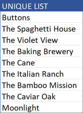
Excel UNIQUE Function: Explained in 4 Minutes

September 29, 2022 by Tyrone Pernsley

The Excel UNIQUE function returns a list of unique values in a list or range.

Note: This function is currently available only to Microsoft 365 subscribers.

To follow along, and for future reference or practice, the file Mike is working from can be found here.

The formula in this video: =UNIQUE(B2:B19)

The tutorial in this video is included in the following interactive workshop: Excel Formulas & Functions 101

Thanks for watching! We’re here to take the fear out of Excel, by empowering you with the essential tools and knowledge necessary for mastering it!

Become a member today: Learn Excel Now All-Access: One-Year Membership

Connect with us on social:
LinkedIn Facebook Twitter

Excel Date Calculations Part 2: Setting Sequential Dates

December 21, 2016 by Tyrone Pernsley

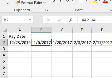
Excel offers a variety of ways to perform date calculations. In part 1 of this series, we showed you how to find the difference between dates. In this week’s post, we cover setting sequential dates in Excel.

Sheryl is getting ready to perform her annual budget. Her job pays her every two weeks. As a result, 10 months of the year, she receives two paychecks, but there are two months where she ends up with three paychecks. She wants to find each payday in the upcoming year and highlight the months where she will receive three checks.

She starts off with her current payday date:

To find the two week pay schedule dates she will:

Enter the formula =A2+14
This yields the next pay day
Then copy the formula across to find all dates
Then look for the date with three in a month and highlight them

In the example, we see that Excel automatically finds the date 14 days from the original date input. In copying the formula across it populates each date two weeks apart.

We at Learn Excel Now hope you now feel confident setting sequential dates in Excel. This process can be used for a variety of business and personal situations.

Like Learn Excel Now? Follow us on social media and share our content with your networks! And don’t forget to sign up for the Newsletter

Kevin – Learn Excel Now

Excel Date Calculations Part 1: Finding the Difference Between Two Dates

December 14, 2016 by Tyrone Pernsley

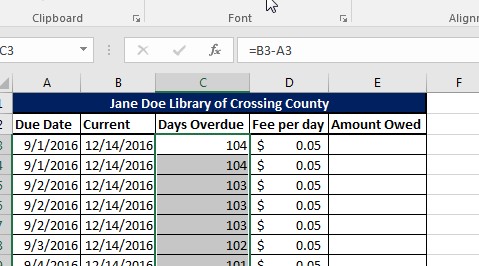
Excel has several built-in date functions you can use to quickly find important information. These are known as Excel date calculations. Today, we will focus on how to find the difference, in number of days, between two different dates. We will also cover how to find a date based on number of days from a given date.

For today’s example, we will use the following spreadsheet outlining due dates for a library:

Here, we have the due date and the current date. To enter the current date into your spreadsheet, you will use the formula =TODAY(). It will autofill with today’s date.

What we don’t have is the number of days overdue, and the overdue fee. To find that, we will:

Subtract the due date from the current date

Multiply the number of days by the fee per day

As you can see, Excel makes it easy to find the exact number of days and then calculate the amount owed. This process involves first finding the number of days and then separately finding the amount due. But you can also build the date calculation right into the fee calculation.

You will use the parenthesis to indicate which function you want performed first (always remember: Excel operates on the Order of Operations).

So, the first part of the calculation will be: =(B3-A3)

Then, tell the formula to also multiply by the amount owed column: =(B3-A3)*D3

Finding a Date Based on Number of Days

Let’s say you had the same spreadsheet, except that the original due date was missing, but you still have the number of days. Your job is to find the original due date. This is basically a reverse of finding the number of days overdue. You will enter:

=B3-C3

This is how you use Excel to find the number of days between two dates or vice versa. Next week, we will cover additional date functions you will want to know. We hope you found today’s lesson on Excel date calculations useful.

Like Learn Excel Now? Follow us on social media and share our content with your networks! And don’t forget to sign up for the Newsletter

Kevin – Learn Excel Now

Excel Formulas: How to Use the LEFT and RIGHT Functions

November 2, 2016 by Tyrone Pernsley

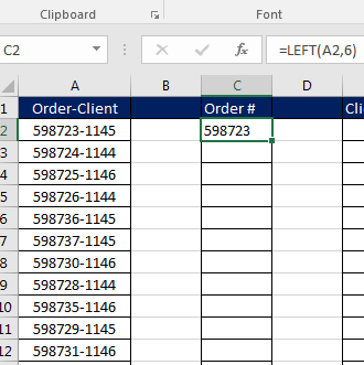
This demonstration covers how to use the LEFT and Right Functions in Excel. These are text functions. In the LEFT function, you can pull a set number of characters out of a cell into another cell starting at the leftmost point. The RIGHT function performs the same except starting at the rightmost point.

Both functions are related to the MID function, which we covered back in September. At the time, one of our customers asked for a demo on the MID function. Since then, we’ve had several follow up requests on the LEFT and RIGHT.

For today’s demonstration, we will be using the following spreadsheet:

In this example, Column A contains a 6-digit number hyphenated with a 4-digit number. The 6-digit number is the order number and the 4 digit is the client ID. Your job is to separate the order number and client ID into Columns C and E, respectively.

How is this done?

For the order number, we will use the LEFT function. We know the code is 6 digits, so we have the number of characters. So in cell C2, you will enter the following formula:

=LEFT(A2,6)

For the client ID, we will use the RIGHT function. In cell E2, you will enter the following formula:

=RIGHT(A2,4)

LEFT Function Syntax:

=LEFT(Destination Cell, Number of Characters)

This tells Excel: Starting on the left of this specified cell, copy to this many characters.

RIGHT Function Syntax:

=RIGHT(Destination Cell, Number of Characters)

This tells Excel: Starting on the right of the specified cell, copy to this many characters.

As you can see in the above demonstration, once the functions have been entered, they can be copied all the way down to finish filling in the data.

We at Learn Excel Now hope you feel comfortable using the RIGHT and LEFT functions.

Like Learn Excel Now? Follow us on social media and share our content with your networks! And don’t forget to sign up for the Newsletter.

Kevin – Learn Excel Now

Essential Excel Functions: How to Use CONCATENATE

July 6, 2016 by Tyrone Pernsley

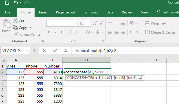
Excel possess many formulas and functions to help you perform essential tasks. The CONCATENATE function is one of most useful. It allows you to combine data from two or more cells into a single string. There are many applications for this function. It is particularly useful when pulling an Excel spreadsheet from a database where pieces of information are broken up over different columns.

To get an idea of how to use this function, let’s take the example of phone numbers. In the following example, the area code, 3-digit prefix and 4-digit ending are all broken up in different columns:

Now, if we want to combine these into a single cell to make the phone numbers easy to view, copy and paste, we will use CONCATENATE. Here is how the formula looks:

= CONCATENATE (Text1,Text2,Text2,…)

Notice you need to identify each individual cell or text making up each component of the function. Here is how it looks when combining the columns to yield the phone numbers:

You can now use the Fill Handle to copy the function all the way down yielding phone numbers in the remaining rows.

Let’s take a look at another example. One of our fans, Susan, brought an interesting query to us a few weeks ago. She was pulling a list of email addresses from her company’s database.

Now, Susan told us that the company’s email worked like this: Firstname.lastname@companydomain.com

As you can see in the image above, the dot between first name and last name and the @ symbol between last name and company domain are missing.

So, to help Susan use the CONCATENATE, we first need to prep the data. Here are the steps to take:

Add a column between First and Last Name
Add a period in the new column – use the Fill Handle to copy it all the way the down
Add a column between Last Name and Company domain
Add the @ symbol and use the Fill Handle to copy it all the way down
In the first open cell in the top row, enter the CONCATENATE function
Use the Fill Handle to copy it all the way down

As you can see in the above image, the function was used successfully to create the email addresses.

We here at Learn Excel Now hope you now feel comfortable using the Excel CONCATENATE function.

Like Learn Excel Now? Follow us on social media and share our content with your networks! And don’t forget to sign up for the Newsletter

Kevin – Learn Excel Now

Excel UNIQUE Function: Explained in 4 Minutes

Excel Date Calculations Part 2: Setting Sequential Dates

Excel Date Calculations Part 1: Finding the Difference Between Two Dates

Excel Formulas: How to Use the LEFT and RIGHT Functions

Essential Excel Functions: How to Use CONCATENATE

Connect with Us

Contact

Connect with Us

Contact

WELCOME BACK!

Reset Password