excel formulas Archives - Learn Excel Now

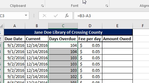
Excel Date Calculations Part 1: Finding the Difference Between Two Dates

December 14, 2016 by Tyrone Pernsley

Excel has several built-in date functions you can use to quickly find important information. These are known as Excel date calculations. Today, we will focus on how to find the difference, in number of days, between two different dates. We will also cover how to find a date based on number of days from a given date.

For today’s example, we will use the following spreadsheet outlining due dates for a library:

Here, we have the due date and the current date. To enter the current date into your spreadsheet, you will use the formula =TODAY(). It will autofill with today’s date.

What we don’t have is the number of days overdue, and the overdue fee. To find that, we will:

Subtract the due date from the current date

Multiply the number of days by the fee per day

As you can see, Excel makes it easy to find the exact number of days and then calculate the amount owed. This process involves first finding the number of days and then separately finding the amount due. But you can also build the date calculation right into the fee calculation.

You will use the parenthesis to indicate which function you want performed first (always remember: Excel operates on the Order of Operations).

So, the first part of the calculation will be: =(B3-A3)

Then, tell the formula to also multiply by the amount owed column: =(B3-A3)*D3

Finding a Date Based on Number of Days

Let’s say you had the same spreadsheet, except that the original due date was missing, but you still have the number of days. Your job is to find the original due date. This is basically a reverse of finding the number of days overdue. You will enter:

=B3-C3

This is how you use Excel to find the number of days between two dates or vice versa. Next week, we will cover additional date functions you will want to know. We hope you found today’s lesson on Excel date calculations useful.

Like Learn Excel Now? Follow us on social media and share our content with your networks! And don’t forget to sign up for the Newsletter

Kevin – Learn Excel Now

Excel Formulas: Using Trace Precedents to Find & Resolve Errors

October 12, 2016 by Tyrone Pernsley

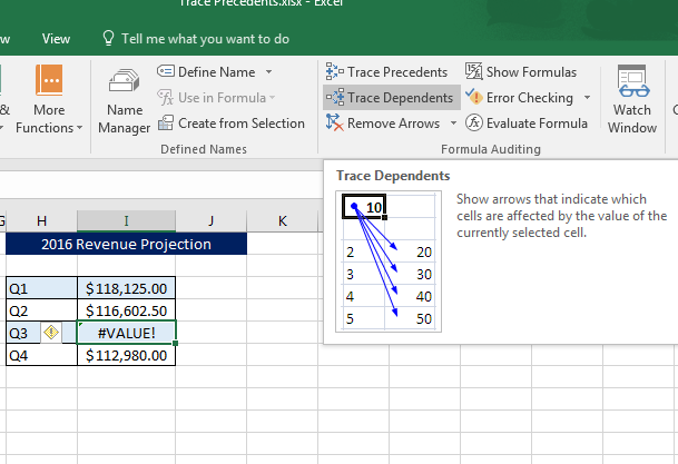
The power of Excel comes from the ability to do complicated calculations using formulas and functions. Sometimes, though, there are errors in formulas that give an error message or return the wrong value. In those instances, Excel also provides tools to resolve errors and check your work. One such tool is trace precedents.

The trace precedents tool finds any and all cells that provide information for the target cell. For example, if you summed up the totals in A1 and B1 into cell C1, both cells A1 and B1 would be precedents for C1.

Some errors in Excel are related to one or more precedent cells giving information that throws off the formula. Trace precedents is a great way to determine if there is a cell causing the issue, and if so, which cell needs to be corrected

For an example of using trace precedents to resolve formula errors, we will use the following spreadsheet:

In this instance, the table is using a simple formula to create revenue projections. The previous year’s quarterly total is increased by the projected growth of 5%. As you can see though, the Q3 project, cell I5, is showing an error message.

So, we will use the trace precedents tool to see if there are any cells causing the issue:

In the demo above, the error was created because one of the cells was incorrect. Instead of the cell containing the percentage amount (5% in cell F4) it was trying to pull the definition of that number one cell above (F3).

The issue could have been caused by simple human error. The person entering the formulas could have simply clicked on the wrong cell.

Once the wrong cell was identified using trace precedents, it was a simple matter of editing the formula to the correct cell and the error was resolved.

There are many instances where this tool could come in handy. Aside from resolving errors, sometimes you might just want to see which cells feed into a formula.

Stay tuned for part 2 next week on Trace Dependents!

We here at Learn Excel Now hope you now feel confident using the trace precedents tool to resolve formula issues.

Like Learn Excel Now? Follow us on social media and share our content with your networks! And don’t forget to sign up for the Newsletter

Kevin – Learn Excel Now

Excel Formula Tricks: Absolute Reference

May 11, 2016 by Tyrone Pernsley

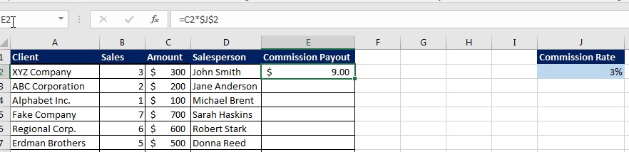
Using Excel to its fullest potential requires knowing how to use formulas. Knowing the different formulas is a great start, but there are tips and tricks you can use to make formulas work even better. In today’s tip, we will explore one of those formula tricks: Absolute Reference aka absolute cell reference.

What is An Absolute Reference in Excel?

This term refers to how you identify the cells being referenced in a formula. A cell reference would be specific cell identified in a formula. For example, if we wanted to run a sum on the following Sale & Tax:

We would enter the following Sum formula:

=sum(A4:B4)

The A4 references the cell with the sale amount and B4 references the cell with the tax amount to give us our total of $318.

Now, if you wanted to copy this formula to find that totals for all of sales, you can copy and paste it down (or use the AutoFill option as in the following animation):

This tool works because of Relative reference. The A4 and B4 in the formula changes to A5 and B5 on row 5, and so on. In this case, the two cells being referenced change according to their relation to where the copied formula is being pasted.

This works well when the information relative to the formula changes in each instance. But what do you do when one of the cells doesn’t change location?

For example, let’s say you wanted to find the commission in the following table by multiplying the sale amount against the commission rate:

This works in the first instance, but then when you try to copy it down, the totals won’t work:

This is because the cell being referenced for the commission rate changes as it is still a Relative Reference.

To make it an Absolute Reference, you use the $ symbol to frame the cell you don’t want to change. Then, when you copy and paste the formula, the commission rate cell stays absolute while the sale remains relative to the row the formula is on:

In this case, the absolute reference anchors one part of the formula so that it can be copied and pasted with ease. This really comes in handy when you have lots of rows of data!

We here at Learn Excel Now hope you enjoyed today’s tip on Excel’s Absolute Reference. This should improve your formulas.

Like Learn Excel Now? Don’t forget to subscribe to our newsletter and follow us on social media!

Kevin – Learn Excel Now

Quick and Easy Math Formulas in Excel: Get Started Now

April 20, 2016 by Tyrone Pernsley

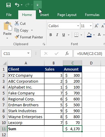
One of the most common uses for Excel is computing large amounts of complex data. Knowing the best formulas to use allows you to crunch those numbers quickly to get the results you need. The formulas you can use vary from simple computation to condition-based criteria. Excel even provides you with specific error messages when data is entered incorrectly. Let’s get started with some of the most used simple formulas.

Most Commonly Used Formulas in Excel

Sum=(cell:cell)

This formula allows you to quickly add numbers in a given range.

$Excel Math Image 1$

Average=(cell:cell)

This formula allows you to find the mean of a given range.

$Excel Math Image 2$

Count=(cell:cell)

This allows you to count the total number of cells in a given range

$Excel Math Image 3$

Using IF Criteria in Excel Formulas

IF Functions allow you to calculate data based on specific criteria.

IF Functions

Evaluates a cell, returns a

true value or returns a false value

In cell H3:

=IF(G3>=20%,”Bonus”,”NA”)

Nested IF

Evaluates multiple criteria, returns a true value or returns a false value

In cell I3:

=IF(G3=10%,”Send Thank You”,IF(G3=15%,”Send Gift”,IF(G3=20%,”Call”,0)))

SUMIF

Evaluates a range of data,

sums if it matches the

criteria. The sum range is the third argument in the

formula.

In cell D7:

=SUMIF(C3:C6,”ABC”,D3:D6)

COUNTIF

Evaluates a range of data,

counts if it matches the criteria.

In cell D8:

=COUNTIF(C3:C6,”ABC”)

AVERAGEIF

Evaluates and averages like

SUMIF.

In cell D9:

=AVERAGEIF(C3:C6,”ABC”,D3:D6)

SUMIFS

A SUMIF with multiple

criteria

In cell D11:

SUMIFS(D3:D6,F3:F6,1200,C3:C6,”ABC”)

COUNTIFS

A COUNTIF with multiple

criteria

In cell D12:

=COUNTIFS(C3:C6,”ABC”,D3:D6,30)

Excel Error Messages

If you enter a formula in Excel that is a circular references or has incomplete data, excel gives you and an error message that identifies the specific problem. You can use that information to correct the problem.

#DIV/0	If you receive this message it is because the formula entered is trying to divide by zero.
#N/A!	This message indicates the formula or a function within the formula cannot find the referenced data.
#VALUE!	This indicates the operand or function used is the wrong type.
#NULL!	This error message occurs when there is a space used in a formula that reference multiple ranges. Use a comma to separate range references.
#NAME?	If the text in the formula is not recognized you will receive this error message.
#REF!	This indicates you used an invalid reference.
#NUM!	This error message occurs when the type of operation in a formula has invalid numeric data.

Here at Learn Excel Now we are committed to helping you do your job better. Please feel free to use these as a quick reference “cheat sheet” when entering formulas in Excel. Determining what formulas work best also depends on your specific needs when using Excel.

If you’re ready to go beyond the basic and start using powerful solutions, you might benefit from this Excel formulas and functions training.

Like these quick and easy tips or have suggestions? Leave your comments below; we’d love to hear from you.

Spread the word and share the knowledge with our social media links!

Kevin – Learn Excel Now.

Excel Date Calculations Part 1: Finding the Difference Between Two Dates

Excel Formulas: Using Trace Precedents to Find & Resolve Errors

Excel Formula Tricks: Absolute Reference

Quick and Easy Math Formulas in Excel: Get Started Now

Sitemap

Connect with Us

Contact