Have you ever had so much data in one cell that that it spills over to the next cell or just disappears? And you don’t want to expand cells because it throws off data presentation in other cells? If you would like to solve this issue, then we are here to help you with wrapping text in Excel!

Like many excel features, there are short and long ways of executing the task. So we will show you both!

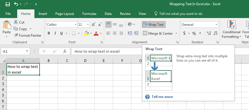
First, a quick way to wrap text for every cell is by going to the “alignment” section of your home toolbar and clicking the icon in the first row, 4^th column.

If you hover over this icon with your mouse you will see it says, “Wrap text”. Click this icon and bam!, now all data will automatically be wrapped to fit the column width

The second way to do this is to first, highlight your desired cell or group of cells. Right click, select “format cells”, chose the “alignment” tab, check off “wrap text”, and click Ok.

If all wrapped text is not visible, it may be because the row is set to a specific height so you may need to play around a little bit to get it to look how you want it too,

The nice part about excel is that you do not have to be afraid of getting your spreadsheet to look how you would like it too. With the text wrapping feature and your prior knowledge of adjusting rows and columns (from our previous post) you have the freedom to customize!

We hope you found today’s quick and easy Excel lesson beneficial. Don’t forget to follow ups on Social Media and subscribe to the blog to get convenient, quick tips like this, and other great Excel training tips so that you can take the fear out of Excel.

Like Learn Excel Now? Sign up for the newsletter!

-Kevin, Learn Excel Now