Learn Excel Now

Conquer the Fear of Excel

  • Home
  • Training
    • Excel
    • MS Office
    • Outlook
    • PowerPoint
    • Word
    • OneDrive
    • Google
  • All-Access
  • eLearning
    • Excel Foundations
    • Micro Courses
      • Simply Excel
  • Resources
  • Login

Excel Basics: How To Separate Text Into Columns

August 22, 2022 by Austin Chia

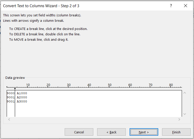
Do you have a list of data that you need to separate into columns in Excel? Maybe you have an address list with the city, state, and zip code all in one column. Or maybe you have a list of product SKUs and want to separate them into individual columns.

Well, before you can start applying all your Excel formulas, you’ll need to get your data all cleaned up. Data is typically cleaned by data engineers but if you’re working with financial data that mostly live within Excel databases, you’ll have to clean it yourself.

In this blog post, I will show you how to use the text to columns wizard in Excel to easily separate text into columns.

I will explain how to use the wizard by both delimiter and fixed width. So whether your data is separated by commas, tabs, or spaces, I will show you how to get it into neat and tidy columns!

Let’s get started!

How Do You Separate Text Into Columns in Excel?

Have you ever tried to filter your data in Excel only to find that all of your data ended up in one column? Before you try out these database tips in Excel, you might want to separate your data into columns first!

It can be frustrating, but luckily there is a tool that can help. The text to columns wizard in Excel allows you to easily separate text into multiple columns.

There are two main ways to use the text to columns wizard: by a delimiter and by fixed width.

If your data is separated by a specific character, such as a comma or tab, then you would use the delimiter option. For example, if your data looks like this:

You would use a comma as your delimiter.

If your data is not separated by a specific character, but you want to split it into columns of equal width, then you would use the fixed width option.

For example, if your data looks like this:

You would use fixed width to split the text into columns.

How To Use The Delimiter Option to Separate Text in Excel

Let’s say you have a list of addresses in one column and you want to separate them into individual columns for the city, state, and zip code. To do this, we would use the delimiter option.

First, highlight the column of data that you want to split. Then, go to the Data tab and click Text to Columns.

In the Convert Text to Columns Wizard, select Delimited and click Next.

On the next page, check the box next to Comma and clear any other boxes that are checked. Then, click Next.

On the next page, you will see a preview of how your data will look when it is split into columns. If everything looks good, click Finish.

And that’s it! Your text should now be split into columns.

End Result

Now that your data is arranged neatly into separate columns, your data format is more suited for further analysis using pivot tables!

How To Use The Fixed Width Option to Separate Text in Excel

If you want to split your text by fixed width, the process is similar. Highlight the column of data that you want to split and go to the Data tab. Click Text to Columns.

In the Convert Text to Columns Wizard, select Fixed Width and click Next.

On the next page, you will see a preview of how your data will look when it is split into columns. Place a break in between each column where you want to split the text. Then, click Next.

On the next page, you will see a preview of how your data will look when it is split into columns. If everything looks good, click Finish.

And that’s it! Your text should now be split into columns.

End Result

I hope this blog post was helpful in showing you how to use the text to columns wizard in Excel. Do consider using this simple but powerful tool in your next data mining or Excel project.

Key Takeaways:

– The text to columns wizard in Excel allows you to easily separate text into multiple columns.

– There are two main ways to use the text to columns wizard: by delimiter and by fixed width.

– If your data is separated by a specific character, such as a comma or tab, then you would use the delimiter option.

– If your data is not separated by a specific character, but you want to split it into columns of equal width, then you would use the fixed width option.

– To use the text to columns wizard, highlight the column of data that you want to split and go to the Data tab. Click Text to Columns. Then, follow the instructions in the wizard.

– Your text should now be split into columns.

Thanks for reading!

Enjoyed this basic tutorial on separating data? Having basic training in Microsoft Excel is important for success in many jobs. If you want to learn more about how to use Excel, check out the other blog posts or sign up for one of our Excel training workshops!

Like Learn Excel Now? Follow us on social media and share our content with your networks! And don’t forget to sign up for the Newsletter

Author Bio

Austin Chia is the Founder of Any Instructor. A data analytics and Excel enthusiast, he seeks to help others learn more about Excel and anything related to analytics and tech. He has experience as a data analyst and data scientist in healthcare and research.

Excel Rank Function: What is It & How to Use It

November 30, 2016 by Tyrone Pernsley

One of Excel’s advanced functions is the RANK function. This formula is used to rank numbers in a dataset by either ascending or descending order.

rank-function-featured-image

Let’s say you were running a customer loyalty program based on earning points. You need to rank customers’ point totals to determine what rewards they receive. You could do a simple sort, but your boss wants the customer names to stay in the same order.

This is the example we will use:

rank-functino-image-1

You will use the RANK function for this challenge, but let’s first explore how the function works.

Syntax of the Rank Function

=RANK(Number, Ref,[Order])

When you use the rank function, your first argument is the number. This is where you specify the cell containing the number you want to be ranked. Next, you identify the range of numbers to be used as the reference (Ref). Finally, you select the order, which is ascending or descending.

Solving the Challenge

So, we will identify B2 as the cell to be used. Then, identify the range as B2 through B11:

rank-function-image-2

Then, select Ascending order and we get our first result:

rank-function-image-3

Before moving onto the remaining lines in the table, we need to add absolute referencing to the range so that it stays consistent while the number being compared changes for each line. A reminder to use the $ between the letter and number of the cell for absolute referencing:

rank-function-image-4

Once you’ve added the absolute reference, you can now copy and paste the formula all the way down to reveal the rank for all lines:

rank-function-image-5

We at Learn Excel Now hope you feel comfortable using the RANK function after this article.

Like Learn Excel Now? Follow us on social media and share our content with your networks! And don’t forget to sign up for the Newsletter

Kevin – Learn Excel Now

All Access Subscription
Our 1-year all-access subscription provides step-by-step guidance for mastering Microsoft Office applications, with workshops, exercises and quick reference eGuides. It's perfect for anyone that needs to brush up on certain skills or even folks who need to learn the programs - from a beginner’s level.
Excel Foundations
Take the fear out of Excel with this 20 module self-paced training course. You will cover the most essential topics to develop a solid foundation of Excel or a lifetime of mastery.

Learn Excel Now helps you conquer the fear of Excel. By providing self-paced and instructor-led training and free strategies and guides, we leave no Excel mystery unsolved.

  • Home
  • Training
  • All-Access
  • Excel Foundations
  • Resources

Connect with Us

  • Facebook
  • Linkedin

Contact

Learn Excel Now
questions@learnexcelnow.com
1-484-259-7664 or 1-800-964-6033
660 American Ave
Suite 203
King of Prussia, PA 19406

Microsoft® Office Excel® is a registered trademark of the Microsoft Corporation in the United States and other countries. All rights reserved.

Copyright © 2023 ­Learn Excel Now

Terms of Service

Privacy Policy

Copyright © 2023 · News Pro Theme on Genesis Framework · WordPress · Log in

WELCOME BACK!

Enter your username and password below to log in

Forget Your Username or Password?

Reset Password

Lost your password? Please enter your username or email address. You will receive a link to create a new password via email.

Log In