
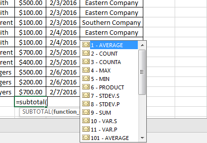
How to Calculate a Subtotal In Excel Using the Filter
Excel has many ways to calculate data. If you know the right formulas and functions, you can find out just about anything you want to…
Excel has many ways to calculate data. If you know the right formulas and functions, you can find out just about anything you want to…
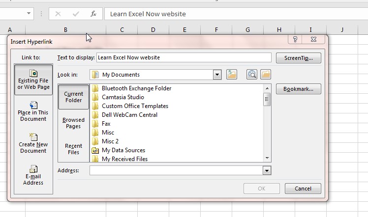
You might already know how to hyperlink a cell to external sources, namely to the web. In case you don’t, here is a quick tutorial…
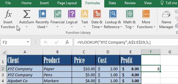
At Learn Excel now, we are always getting questions about VLookUp. Making sense of VLookUp requires breaking the function down and understanding the key…

Clean, readable data makes Excel much easier to use. A common struggle is how to remove duplicates in Excel. Having too many duplicates causes inaccuracies…
Please confirm you want to block this member.
You will no longer be able to:
Please note: This action will also remove this member from your connections and send a report to the site admin. Please allow a few minutes for this process to complete.