Excel Analytics: Creating Tables for Your data

There are a variety of ways to sort and organize your data in Excel. These features allow you to quickly process data to get essential analytics, statistics, trends and other information to inform decision-making. One feature is using Excel tables. Excel Tables are great way to quickly and easily organize and display your data. The following quick guide will provide you with tips, so you can start creating Tables for your data.

Creating a Table

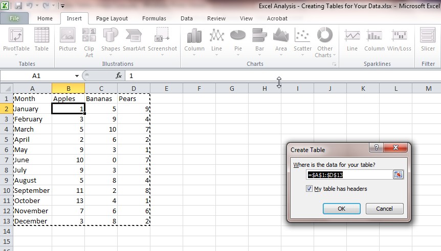
To create a table, first highlight the data that you want included, then go to the “Insert” tab on the top toolbar and select “Table.”

Your table will be created, and you will automatically be in the “Design” tab.

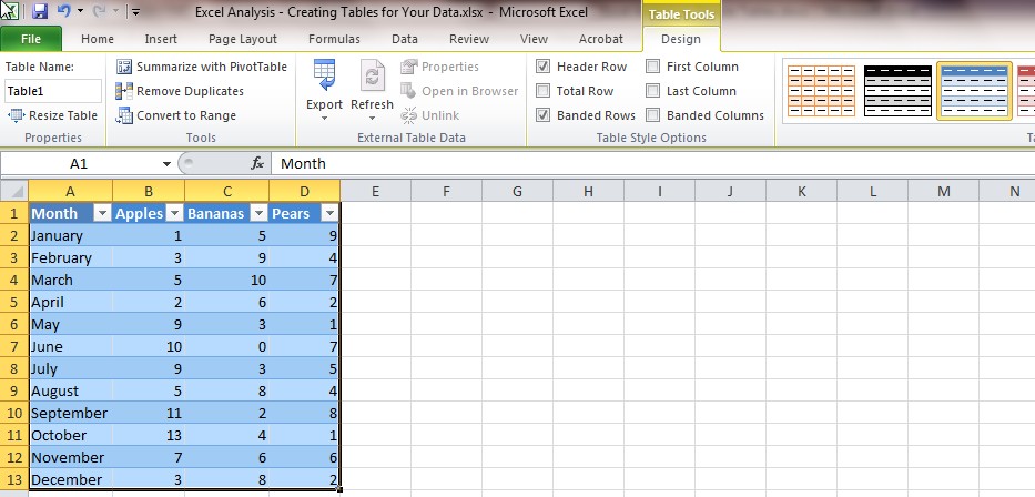
Now, you can choose how you want your table to look by choosing from the different table styles. You can choose from a variety of different colors and then you can choose color density from light to dark. There is also a quick shortcut that you can use to insert a table. To use this, highlight your data, and then click “Ctrl” + “L.” Your table will be created automatically and then you can design it.

Filtering and Sorting the Data in Your Table

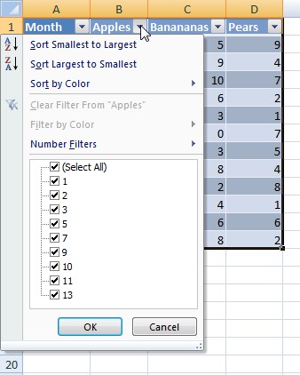
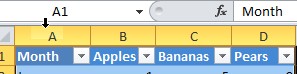Once you have created your table, each column heading will have a drop-down box that automatically appears in the column heading in the top row. The down arrow key allows you to open the drop-down menu.

You have different options to sort the data in the drop-down box. From there, you can sort the data alphabetically, by highest or lowest value or by color.

To filter your data, you can customize number or text filters by specifying the values that you want hidden or shown. You can also exclude values that you don’t want show by unchecking the check box next to the value(s) that you want hidden.

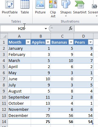
Making Calculations in Your Table

You can use calculations to find the totals, averages, and various other calculations for columns or rows. To do this, you have two options. First option: you can click on the cell at end of the column or row and click on the “AutoSum” button.

The other option is to select the cell at the end of the column or row, then go to the “Formulas” tab and select the formula that you want to use. When the formula is added to the table, a drop-down arrow is automatically inserted to the right of the value. From the drop-down options, you can choose different formulas to perform other calculations on that row or column.

We here at Learn Excel Now hope you now feel confident in creating tables for your data in Excel. It is our desire to bring you the best advice possible to effectively and efficiently use your desktop features so you can focus on your work. Subscribe to our blog to receive weekly Excel tips. If you’re looking for more in-depth training check out our upcoming instructor-led, live online training.

Liked this Excel Tables quick guide? Have questions? Leave your comments below; we’d love to hear from you.

Getting Social with Excel: Spread the word and share the knowledge!

Kevin – Learn Excel Now