Creating 3-D Formulas in Excels for Multiple Worksheets

A 3-D formula in Excel can be used to calculate data using multiple worksheets in a workbook. Check out these tips to learn how to create and use 3-D formulas in Excel.

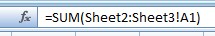
What 3-D Formulas in Excel  Look Like

The syntax for a 3-D formula is “worksheetA:worksheetB!reference”

• WorksheetA is the first worksheet that you want to be included in the calculation.
• WorksheetB is the last worksheet that you want included in the calculation.
• The reference is the cell or cells that contain the values that you want to be a part of the calculation.

Functions that You Can Use with 3-D Formulas

• SUM: This calculates the sum of all the values you select
• AVERAGE: This calculates the average of all the values you select
• COUNT: This counts the number of cells in the range that contain numbers
• MAX: This returns the largest value in the set of values that you select
• MIN: This returns the smallest value in the set of values that you select
• PRODUCT: This multiplies all the numbers that you select
• STDEV: This estimates the standard deviation based on a sample
• VAR: This estimates the variance based on a sample
• VARP: This calculates the variance based on the entire population

Creating 3-D Formulas in Excel

To create a 3-D formula, first select the cell where you want to enter the function. Now, on the “Formula” tab, select the function that you want to use. From there, you will need to select the data that you want to be included in the calculation. First, click on the sheet for the first worksheet that you want to reference, then hold the “Shift” key and click on the last sheet that you want included. Now you will need to highlight the cell(s) that should be a part of the calculation. Make sure that the values are in the same location on all of the worksheets that you are using. When you are finished selecting your sheets and cells, click “Enter” and your function will be calculated based on the data you selected.

3-D Formulas Shortcut for Adding Values

To quickly calculate a sum with a 3-D formula, you can use this shortcut. In the worksheet that you want your data to be calculated in, select a cell and click “AutoSum.” Click on the first worksheet that contains the data that you want calculated then hold down the “Shift” and click on the last worksheet that you want to be included in the calculations. Finally click on a cell that you want the calculation to be calculated from, and press “Enter.” Your solution will appear in the cell that you clicked on originally.

Liked this Excel combined charts guide? Have questions? Leave your comments below; we’d love to hear from you.

Getting Social with Excel: Spread the word and share the knowledge!

Kevin – Learn Excel Now