Making Sense of VLookUp: Quick and Easy Tips

At Learn Excel now, we are always getting questions about VLookUp. Making sense of VLookUp requires breaking the function down and understanding the key components and what you are trying to find.

What is VLookup?

The VLookup function allows you to find data that is stored in a table from another spreadsheet or a smaller table.

There are 2 ways to enter the VLookUp Function:

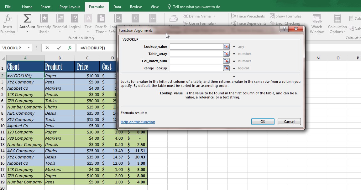
1. Go to the Formulas Tab, click the “Lookup & Reference” dropdown and select Vlookup. This will open the following dialogue box:
2. You can enter the function as a formula:
   =VLOOKUP(lookup_value, table_array, col_index_num, [range_lookup = TRUE])

Syntax of the VLookup Function:

Lookup_value: The value to search in the first column of the table. This can be a reference or a value.
Table_array: This is two or more columns of data. You can use a reference to a range or a range name. The values that appear in the first column are those searched by the lookup_value. These values can take many forms including text, numbers, or logical values.
Col_index_num: This is the table from which the matching value is returned. There are several different scenarios for the value’s placement:

• If the col_index_num is less than 1, then the vlookup shows the error “#Value!”
• If the col_index_num is greater than the number of columns in the table_array, then the vlookup shows the error “#REF!”
• If the col_index_num is 1, then the value will be in the first column of the table_array.
• If the col_index_num is 2, then the value will be in the second column of the table_array (and so on)

Range_lookup: This function is meant to specify whether vlookup should find an exact or approximate match of the value you search.

• If “true” or 1 is used, then an exact is returned unless there is not an exact match, in which case the next largest value that is less than the lookup_value is returned.
• If “false” or 0 is used, then an exact match is returned. If there are two or more values that are an exact match, the first value found is used. If no exact match is found then the error “#N/A” is returned

S0, what does that all mean?

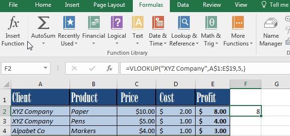
Let’s say you wanted to find the total profits from sales to XYZ Company in the following table:

Now, in this simple table, you could just sum the individual cells under the Profit heading that correspond to XZY Company. But, if this table were hundreds of rows long, that would be impractical.

So, we are going to use VLookUp:

=VLOOKUP(“XYZ Company”,A1:E19,5,)

In this formula:

XYZ Company Acts as the Lookup_value
A1:E19 is the table_array
5 is the col_index_num
Because we are just looking to return a value, there is no Range_lookup required.

Other Helpful Tips:

• You need to use “Ctrl,” “Shift,” and “Enter” to create brackets around an array formula rather than simply using “Enter.”
• Keep in mind that table_array doesn’t differentiate between uppercase and lowercase letters.
• Put the value of the first column of the table_array in ascending sort order to ensure that vlookup gives you the correct value. To set this, click on the “Data” icon on the tool bar, then select “Sort,” and finally select “Ascending.”
• If you get the error message “#N/A”, check to make sure that the lookup_value is not smaller than the smallest value in the first column of the table_array.

We here at Learn Excel Now hope you now feel more comfortable using VLookUp. It is one of the most widely used Excel functions but it is a complicated tool. Making sense of VlookUp requires practice and use.

Like Learn Excel Now? Follow our social media pages and share our Excel content with your networks!

Kevin – Learn Excel Now