
Excel Pivot Tables: Using Slicers to Filter Data
Are you looking for a way to filter your Excel pivot tables quickly? If so, then you need to learn about slicers! Slicers are a great way to control the data that is displayed in your pivot table.
In this blog post, we will introduce you to pivot table slicers and show you how to use them through a step-by-step tutorial.
So, if you want to learn how to use slicers with pivot tables, keep reading!
What Are Pivot Table Slicers?
Pivot table slicers are a new feature only found in versions from Excel 2010 onward. They allow you to quickly filter pivot table data by clicking on a value in the slicer.
Why Use Pivot Table Slicers?
Pivot table slicers are a great way to filter pivot table data in Excel. Slicers are an alternative to the default filters in Excel.
They are easy to use and they provide a quick way to change the data that is displayed in your pivot table. You’ll be able to mine data for useful business insights.
Another advantage of using slicers is that they can be used to filter multiple pivot tables at the same time. This is because slicers are connected to pivot tables.
Therefore, if you have multiple pivot tables in your workbook, you can use a slicer to filter all of them at the same time. This can save you a lot of time if you need to regularly filter pivot table data.
When Should Pivot Table Slicers Be Used?
Pivot table slicers should be used when you need to quickly filter pivot table data. They are handy if you have multiple pivot tables in your workbook.
They’re also a great way to filter data when creating an Excel dashboard for your Excel project.
With the use of pivot table slicers in Excel, you’ll get to dig deeper into your data and visualize them better through charts.
Although not as powerful as the filters available in other data analysis tools like Tableau, slicers are easy to create and implement in your work!
How Do Pivot Table Slicers Work?
Pivot table slicers work by connecting to pivot tables. When you create a slicer, you need to specify which pivot table it should be connected to. Once a slicer is connected to a pivot table, it can be used to filter the data in that pivot table.
If you have multiple pivot tables in your workbook, you can connect a slicer to all of them. This will allow you to quickly filter the data in all of the pivot tables at the same time.
How To Use Pivot Table Slicers to Filter Data
Now that you know the basics of using pivot table slicers, let’s take a look at how to use them with a pivot table. We will walk you through the process step-by-step so that you can see how it’s done.
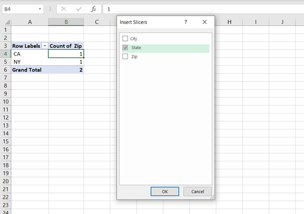
To start, select the pivot table with which you want to use the slicer. Then, click on the “Insert” tab and then click on “Slicer.”
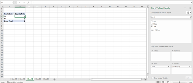
In the “Select a slicer” window, select the field that you want to use as a slicer. For this example, we will use the “State” field.
Next, click “OK.” Your pivot table should now have a slicer associated with it. To use the slicer, simply click on the items that you want to include in your pivot table.
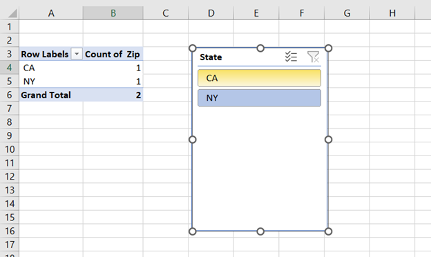
For example, if you only want to see data for the states of “CA” only, click on “CA”. The pivot table will update to only include data for that state.
And if you want to filter and include bot, hold Shift and click both “CA” and “NY”. The pivot table will update to only include data for those two states.
By using this slicer, you’re able to quickly switch between states by selecting the values you need. This can be great when presenting important data using your pivot table.
Rather than just using the regular filters in the pivot table slicers give you a more intuitive way to interact with your data!
Having this knowledge of using slicers in your pivot tables is an essential skill in data analytics in business, where presentation summaries are used in day-to-day operations.
Key Takeaways:
- Pivot table slicers are a great way to quickly filter pivot table data.
- They’re easy to use and can be connected to multiple pivot tables.
- You can use them to filter data by region, sales, criteria, etc.
Conclusion
As you can see, pivot table slicers are a great way to quickly filter your data. So, if you haven’t already started using them, we encourage you to do so!
Thanks for reading!
Enjoyed this basic tutorial on separating data? Having basic training in Microsoft Excel is important for success in many jobs. If you want to learn more about how to use Excel, check out the other blog posts or sign up for one of our Excel trainings!
Like Learn Excel Now? Follow us on social media and share our content with your networks! And don’t forget to sign up for the Newsletter
Author Bio
Austin Chia is the Founder of Any Instructor. A data analytics and Excel enthusiast, he seeks to help others learn more about Excel and anything related to analytics and tech. He has experience as a data analyst and data scientist in healthcare and research.