
Excel Conditional Formatting: Quick Tips to Get Started
Using Excel in the workplace, or for personal needs, is made much simpler when you know who to use all of the tools and features effectively. This week, Learn Excel Now brings you our tips for using Excel conditional formatting. The conditional formatting tool in Excel allows you to apply many different formatting options (such as background colors, borders, and font formatting) to data that meets certain conditions. This makes sorting and recognizing data easier.
In order to set a formatting condition, first select the cells that you want to format. Then on the “Home” tab, click “Conditional Formatting” in the “Style” section. See the image below for a reference point.

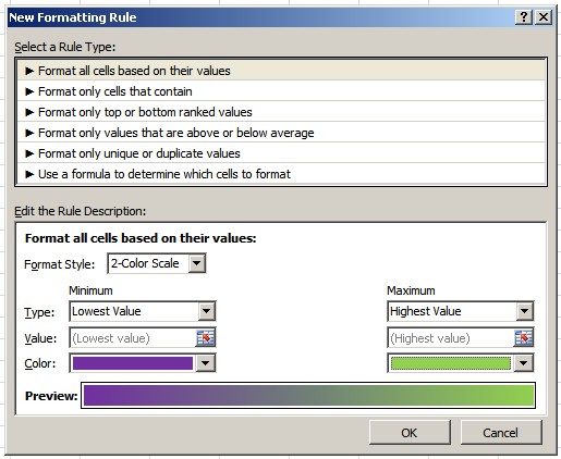
For the next step in the process, choose “New Rule.” From there you can select from the following rule types:
- Format all cells based on their values: With this rule you can choose a 2 or 3 color scale to show which category that value fits closest to (lowest value, percentage, formula, etc). You can also choose from a data bar or icon sets that you can specify the rules of.
- Format only cells that contain: With this rule, you can pick a certain format for cells that have a certain value between, greater than, equal to, etc. to a certain value.
- Format only top or bottom ranked values: With this rule, you can format values that are in the top or bottom percentage of the range.
- Format only values that are above or below average: With this rule, you can format the cells that are above or below the average of the range.
- Format only unique or duplicate values: With this rule, you can format the cells that contain a duplicate or unique value.
- Use formula to determine which cells to format: With this rule, you can format cells that contain a certain formula.

After creating the rule, it will apply immediately. Any cell that fits the rule will take on the specified format. If none of the cells changed, that means that your rule didn’t apply to any of them. But, as soon as you enter a value that meets the rule, it will take on the specified format.
We here at Learn Excel Now hope you now feel confident in your ability to apply Excel conditional formatting to your spreadsheets. It is our desire to bring you the best advice possible to effectively and efficiently use your desktop features so you can focus on work. Subscribe to our blog to receive weekly Excel tips.
Liked this Excel conditional formatting guide? Have questions? Leave your comments below; we’d love to hear from you.
No anyone else who could use these tips? Feel free to share!
Kevin – Learn Excel Now
Responses